Today, I will introduce to you about using the Pandas library.
The goals of this article include:
- Create Series and DataFrame data structures
- Use pandas mathematical functions, as well as
broadcasting features - Use the Pandas library to import and manipulate data
What is pandas?
The Pandas library is built on NumPy and provides easy-to-use data structures and data analysis tools for the Python programming language.
When you want to use a simple declaration like this:
1 2 | <span class="token keyword">import</span> pandas <span class="token keyword">as</span> pd |
The series data structure
The series is one of the main data structures of Pandas. You can think of it as a combination of List and Dictionary of Python. All data is stored in order and has a label so you can call them. A Pandas Series is a one-dimensional labeled array capable of containing any type of data with axial or index labels. An easy way to imagine, we have data consisting of 2 columns. The first column is Index, which is like Keys in Dictionary. The second column is data. We must note that the data column has its own label and can be called with the .name attribute. This is different from Dictionary and is useful when it consolidates with multiple columns of data. 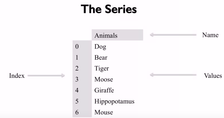
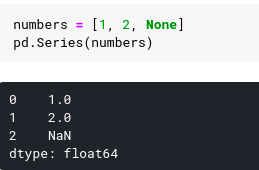
We can instantiate a series by passing a list of values. The panda function will then automatically assign an index starting with 0 and name the string None. For example : 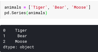
We see here the pandas function automatically determines the data type held in the list, in the example above we did it in the list of string and the pandâ function sets the type to ‘object’.
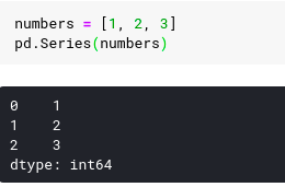
If we did a list of all numbers like the following example, the panda would set the type to int64 .
Below the panda function stores the values entered in the series using the numpy library. This provides increased speed when processing data compared to traditional python List.
There are several types of details that exist for performance that are important to know. The most important is how numpy and the panda function handle the missing data. In phyton we have the none type to indicate missing data. But what do we do if we want to have a stylesheet like we do in a bunch of objects?
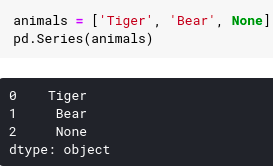
Underneath the panda function does some kind of conversion. If we create the list string and we have an element, a type of None , the panda function inserts it as None and uses this type of object for the underlying row.
If we create a list of numbers, integers, and set them to None, the panda function automatically converts this to a special dynamic numerical value specified as NaN, which stands for not a number.
NaN is not None and when we try to test it is wrong. We cannot automatically do NaN checks with itself. When we do, the answer is always wrong. We need to use special functions to check.
1 2 3 4 5 | <span class="token keyword">import</span> numpy <span class="token keyword">as</span> np np <span class="token punctuation">.</span> nan <span class="token operator">==</span> <span class="token boolean">None</span> <span class="token comment"># False</span> np <span class="token punctuation">.</span> nan <span class="token operator">==</span> np <span class="token punctuation">.</span> nan <span class="token comment"># False</span> np <span class="token punctuation">.</span> isnan <span class="token punctuation">(</span> np <span class="token punctuation">.</span> nan <span class="token punctuation">)</span> <span class="token comment"># False</span> |
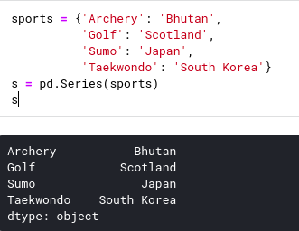
A series can be created from dictionary . If we create this way, the index is automatically assigned as the dictionary key that we have provided and not the indexes as above. For example:
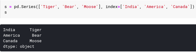
We can also initialize the index by passing the index as a list string as follows:
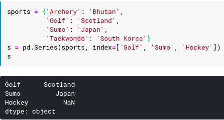
What happens if our list of index values is not associated with the dictionary key ? The panda function will take only the key words whose index values are passed. For example:
Querying a Series
A panda Series function can be queried by index or index label . As we saw above, if we didn’t give an index to series, index and label are the same values. To query by locating numbers starting at 0, use the iloc attribute. To query the label index , we can use the attribute ‘loc’. We have the following example:
1 2 3 4 5 6 7 8 9 | sports <span class="token operator">=</span> <span class="token punctuation">{</span> <span class="token string">'Archery'</span> <span class="token punctuation">:</span> <span class="token string">'Bhutan'</span> <span class="token punctuation">,</span> <span class="token string">'Golf'</span> <span class="token punctuation">:</span> <span class="token string">'Scotland'</span> <span class="token punctuation">,</span> <span class="token string">'Sumo'</span> <span class="token punctuation">:</span> <span class="token string">'Japan'</span> <span class="token punctuation">,</span> <span class="token string">'Taekwondo'</span> <span class="token punctuation">:</span> <span class="token string">'South Korea'</span> <span class="token punctuation">}</span> s <span class="token operator">=</span> pd <span class="token punctuation">.</span> Series <span class="token punctuation">(</span> sports <span class="token punctuation">)</span> <span class="token keyword">print</span> <span class="token punctuation">(</span> s <span class="token punctuation">.</span> iloc <span class="token punctuation">[</span> <span class="token number">3</span> <span class="token punctuation">]</span> <span class="token punctuation">)</span> <span class="token comment"># 'South Korea'</span> <span class="token keyword">print</span> <span class="token punctuation">(</span> s <span class="token punctuation">.</span> loc <span class="token punctuation">[</span> <span class="token string">'Golf'</span> <span class="token punctuation">]</span> <span class="token comment"># 'Scothland'</span> <span class="token keyword">print</span> <span class="token punctuation">(</span> s <span class="token punctuation">[</span> <span class="token number">3</span> <span class="token punctuation">]</span> <span class="token punctuation">)</span> <span class="token comment"># 'South Korea'</span> |
With the two ways below you see above, it is understandable that the pandas function tries to generate readable code and provide intelligent types of syntax using index operators directly on strings. For example, if we pass an integer, the operator will act as if you want to query through the iloc attribute. If we pass a ‘string’ object, it will query as if you want to use the ‘loc’ attribute based on the label.
What happens if our index is an integer list? This is a bit complicated and the panda function cannot determine automatically whether you are planning to query using an index location or an index label. So one needs to be careful when using index operators on series itself. And the safest option is to use iloc or loc . For example, we want to access the first element:
1 2 3 4 5 6 7 8 | s <span class="token operator">=</span> <span class="token punctuation">{</span> <span class="token number">99</span> <span class="token punctuation">:</span> <span class="token string">'a'</span> <span class="token punctuation">,</span> <span class="token number">100</span> <span class="token punctuation">:</span> <span class="token string">'b'</span> <span class="token punctuation">,</span> <span class="token number">101</span> <span class="token punctuation">:</span> <span class="token string">'c'</span> <span class="token punctuation">,</span> <span class="token number">102</span> <span class="token punctuation">:</span> <span class="token string">'d'</span> <span class="token punctuation">}</span> s <span class="token operator">=</span> pd <span class="token punctuation">.</span> Series <span class="token punctuation">(</span> s <span class="token punctuation">)</span> <span class="token keyword">print</span> <span class="token punctuation">(</span> s <span class="token punctuation">[</span> <span class="token number">0</span> <span class="token punctuation">]</span> <span class="token punctuation">)</span> <span class="token comment"># lỗi </span> <span class="token keyword">print</span> <span class="token punctuation">(</span> s <span class="token punctuation">.</span> iloc <span class="token punctuation">[</span> <span class="token number">0</span> <span class="token punctuation">]</span> <span class="token punctuation">)</span> <span class="token comment"># 'a'</span> |
Now we know how to get data out of a series. Now, let’s focus on working with data. Some common tasks are to look at data inside the series and do some math. Similar to the NumPy library, the Pandas below supports a calculation method called vectorization .
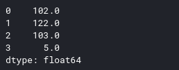
For example, calculating the numbers in the series we do the following:
1 2 3 4 | s <span class="token operator">=</span> pd <span class="token punctuation">.</span> Series <span class="token punctuation">(</span> <span class="token punctuation">[</span> <span class="token number">100.00</span> <span class="token punctuation">,</span> <span class="token number">120.00</span> <span class="token punctuation">,</span> <span class="token number">101.00</span> <span class="token punctuation">,</span> <span class="token number">3.00</span> <span class="token punctuation">]</span> <span class="token punctuation">)</span> total <span class="token operator">=</span> np <span class="token punctuation">.</span> <span class="token builtin">sum</span> <span class="token punctuation">(</span> s <span class="token punctuation">)</span> <span class="token keyword">print</span> <span class="token punctuation">(</span> total <span class="token punctuation">)</span> <span class="token comment"># 324</span> |
Next add 2 to the value of each row as follows:
1 2 3 | s <span class="token operator">+=</span> <span class="token number">2</span> <span class="token comment">#adds two to each item in s using broadcasting</span> s <span class="token punctuation">.</span> head <span class="token punctuation">(</span> <span class="token punctuation">)</span> |
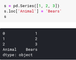
We can also add a new value just by calling the .loc index operator:
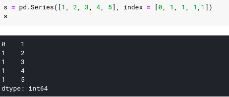
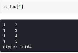
We have found that matching types for data value types or index labels do not matter to Pandas. As in the examples above, each data has only 1 unique index, we have an example where the font index values must not be unique:
The next part we will learn about DataFrame, which is similar to the series object but consists of data columns and is the structure we will spend time working upon cleaning and aggregating data.
The DataFrame Data Structure
DataFrame data structure is the focus of panda library. It is an important part that we will work on in data analysis and data cleaning tasks. DataFrame is the concept of a 2-dimensional series object, has an index and columns, each column has a label. In fact, the difference between a column and a row is only conceptual. We can consider DataFrame as an array labeled two axes. 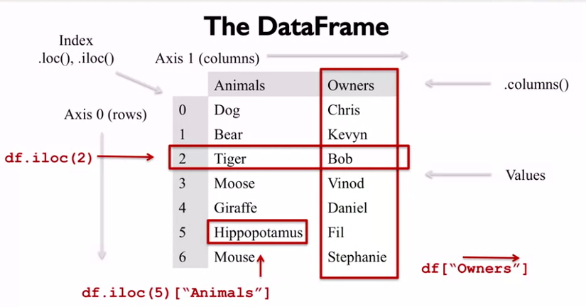
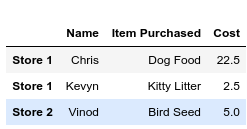
We can create DataFrame in many different ways. For example, we can use a group of series , each series represents a row of data, or we can use a group of dictionary , each dictionary represents a row of data. We have the following example:
1 2 3 4 5 6 7 8 9 10 11 12 13 | <span class="token keyword">import</span> pandas <span class="token keyword">as</span> pd purchase_1 <span class="token operator">=</span> pd <span class="token punctuation">.</span> Series <span class="token punctuation">(</span> <span class="token punctuation">{</span> <span class="token string">'Name'</span> <span class="token punctuation">:</span> <span class="token string">'Chris'</span> <span class="token punctuation">,</span> <span class="token string">'Item Purchased'</span> <span class="token punctuation">:</span> <span class="token string">'Dog Food'</span> <span class="token punctuation">,</span> <span class="token string">'Cost'</span> <span class="token punctuation">:</span> <span class="token number">22.50</span> <span class="token punctuation">}</span> <span class="token punctuation">)</span> purchase_2 <span class="token operator">=</span> pd <span class="token punctuation">.</span> Series <span class="token punctuation">(</span> <span class="token punctuation">{</span> <span class="token string">'Name'</span> <span class="token punctuation">:</span> <span class="token string">'Kevyn'</span> <span class="token punctuation">,</span> <span class="token string">'Item Purchased'</span> <span class="token punctuation">:</span> <span class="token string">'Kitty Litter'</span> <span class="token punctuation">,</span> <span class="token string">'Cost'</span> <span class="token punctuation">:</span> <span class="token number">2.50</span> <span class="token punctuation">}</span> <span class="token punctuation">)</span> purchase_3 <span class="token operator">=</span> pd <span class="token punctuation">.</span> Series <span class="token punctuation">(</span> <span class="token punctuation">{</span> <span class="token string">'Name'</span> <span class="token punctuation">:</span> <span class="token string">'Vinod'</span> <span class="token punctuation">,</span> <span class="token string">'Item Purchased'</span> <span class="token punctuation">:</span> <span class="token string">'Bird Seed'</span> <span class="token punctuation">,</span> <span class="token string">'Cost'</span> <span class="token punctuation">:</span> <span class="token number">5.00</span> <span class="token punctuation">}</span> <span class="token punctuation">)</span> df <span class="token operator">=</span> pd <span class="token punctuation">.</span> DataFrame <span class="token punctuation">(</span> <span class="token punctuation">[</span> purchase_1 <span class="token punctuation">,</span> purchase_2 <span class="token punctuation">,</span> purchase_3 <span class="token punctuation">]</span> <span class="token punctuation">,</span> index <span class="token operator">=</span> <span class="token punctuation">[</span> <span class="token string">'Store 1'</span> <span class="token punctuation">,</span> <span class="token string">'Store 1'</span> <span class="token punctuation">,</span> <span class="token string">'Store 2'</span> <span class="token punctuation">]</span> <span class="token punctuation">)</span> df <span class="token punctuation">.</span> head <span class="token punctuation">(</span> <span class="token punctuation">)</span> |
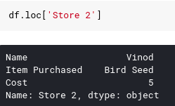
Similar to series , we can extract data using iloc and loc properties. Because the DataFrame is bidirectional, executing an application with the lock operator will return 1 series as a row. For example, if we want to retrieve the data of Store 2 , we do the following, note that the name of the series will return to the index of the row, while the results include the name column:
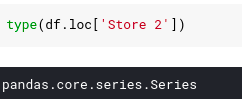
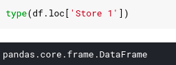
We can check the returned data type by using the type function in python.
An important thing to remember is that the index and column names may not be unique. For example:
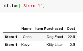
In the example above, we see 2 records for Store 1 purchases are different goods. If we use a single value with the Lock property of DataFrame , many rows of DataFrame are returned then it is not a new Series but a new DataFrame .
One of the features of Panda's DataFrame is that we can quickly select data sets on multiple axes. For example, if we want the price list of store 1, we will provide two parameters to .loc , one is the row index, 1 is the column name as follows:
1 2 | df <span class="token punctuation">.</span> loc <span class="token punctuation">[</span> <span class="token string">'Store 1'</span> <span class="token punctuation">,</span> <span class="token string">'Cost'</span> <span class="token punctuation">]</span> |
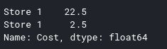
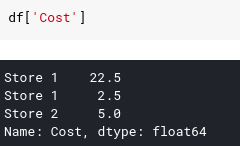
What if we just want to select the column and get a list of all expenses? The simplest way would be as follows:
It works but it’s pretty bad, since iloc and loc are used for row selection, so Pandas developers use the DataFrame direct index DataFrame for column selection, because the columns always have names. As these are familiar with relational databases, this operator is similar to column mapping.
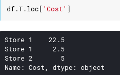
Finally, because the result of using the index operator is DataFrame or Series we can deep chain operators together. For example, we can rewrite the query for query cost list of store 1 as follows:
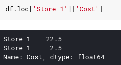
This looks pretty reasonable and gives us the results we want. But chain worms can come at a cost and are best avoided if you can use a different approach. Specifically, string worms tend to cause the panda function to return a copy of the DataFrame instead of a view of the DataFrame . With retrieving data, this is not a big problem although it may be slower than necessary. If you are changing data, this is an important difference and may be the reason for the error. Here is another method:
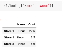
As we see .loc does a row selection and it can take two parameters, row index and column name list. .loc also supports slicing . If we want to select all rows, we can use a column to specify a full array from start to finish. Then add the column name as the second parameter as a string. In fact if we want to include multiple columns, we can do it in a list. And panda will bring back the columns we requested.
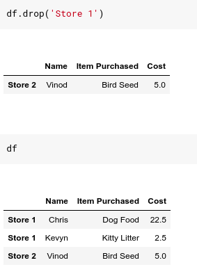
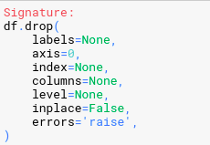
Now before we stop discussing data access in DataFrame , let’s talk about data removal. It’s easy to delete data in Series and DataFrame and we can use the drop function to do that. . The delete function does not change the data frame by default. Instead return you a copy of the data frame with the rows removed. We can see that our original data frame is still intact.
The Drop function has many parameters to choose from, of which the two parameters we should care about, the first is the inplace , it is set to False , the DataFrame has updated in place or a copy will be returned. The second parameter is axis – the axis that we will delete. The default is 0 for the row axis, but we can change it to 1 if we want to delete the row. The parameters in the Drop function are as follows:
The second way to delete a column is through the use of the index operator, using the del keyword. How to delete this data, however, it affects immediately on DataFrame and does not return a 1 View result (I explained the concept of view and coppy in NumPy article).
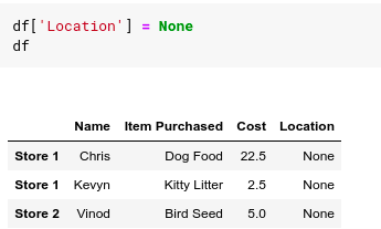
Finally, adding a new column to the DataFrame is as easy as assigning it to some values. For example, if we want to add a new Location as a column with the default value of None .
Dataframe Indexing and Loading
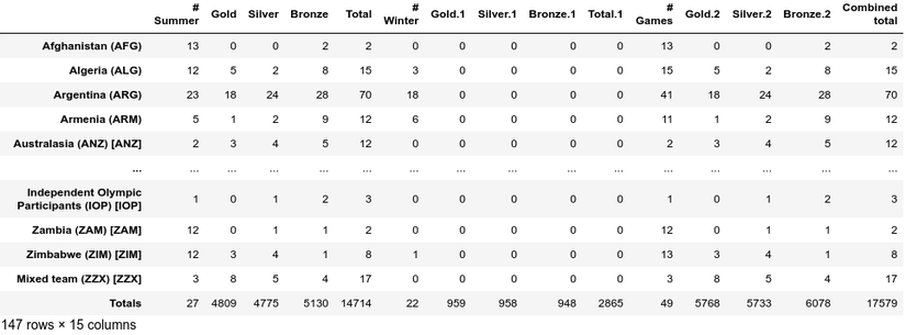
A common workflow is to read data into a DataFrame and then reduce this data frame with specific columns or rows that interest you. In this article, we will mainly use medium or smaller sized data sets. In this section, we will work with the olympics.csv file, which is data from wikipedia containing a summary list of the medal winners of the Olympics. We can read this file in DataFrame by calling read_csv , the command df.head () will output the first 5 parts.
1 2 3 | df <span class="token operator">=</span> pd <span class="token punctuation">.</span> read_csv <span class="token punctuation">(</span> <span class="token string">'olympics.csv'</span> <span class="token punctuation">)</span> df <span class="token punctuation">.</span> head <span class="token punctuation">(</span> <span class="token punctuation">)</span> |
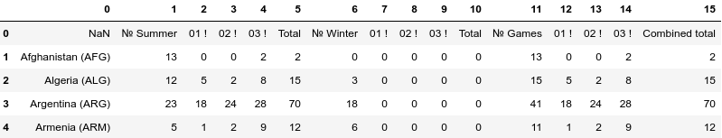
When we look at the DataFrame , we see that the first part has the part from NaN in it. Because it is a blank value and the rows are automatically indexed for us. It is clear that the first row of data in the DataFrame is what we really want to see as column names, and the first column in the data is the name of the countries, which we want is the index column. We will do the following:
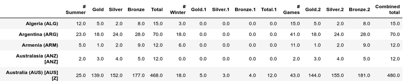
1 2 3 | df <span class="token operator">=</span> pd <span class="token punctuation">.</span> read_csv <span class="token punctuation">(</span> <span class="token string">'olympics.csv'</span> <span class="token punctuation">,</span> index_col <span class="token operator">=</span> <span class="token number">0</span> <span class="token punctuation">,</span> skiprows <span class="token operator">=</span> <span class="token number">1</span> <span class="token punctuation">)</span> df <span class="token punctuation">.</span> head <span class="token punctuation">(</span> <span class="token punctuation">)</span> |
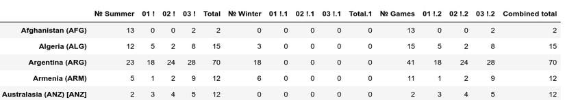
Now, this data comes from all Olympics medal tables on wikipedia. If we look at the columns we can see instead of writing the gold, silver and bronze medals whose data reads “01!”, “02!”, “03!”. So we will clean the data, we can do this by editing on the .csv file directly but we can also name the columns using Pandas.
Panda stores a list of all the columns in the .columns attribute.
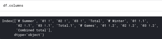
We can change the values of the name columns by repeating this list and using the rename method of the DataFrame as follows:
1 2 3 4 5 6 7 8 9 10 11 12 | <span class="token keyword">for</span> col <span class="token keyword">in</span> df <span class="token punctuation">.</span> columns <span class="token punctuation">:</span> <span class="token keyword">if</span> col <span class="token punctuation">[</span> <span class="token punctuation">:</span> <span class="token number">2</span> <span class="token punctuation">]</span> <span class="token operator">==</span> <span class="token string">'01'</span> <span class="token punctuation">:</span> df <span class="token punctuation">.</span> rename <span class="token punctuation">(</span> columns <span class="token operator">=</span> <span class="token punctuation">{</span> col <span class="token punctuation">:</span> <span class="token string">'Gold'</span> <span class="token operator">+</span> col <span class="token punctuation">[</span> <span class="token number">4</span> <span class="token punctuation">:</span> <span class="token punctuation">]</span> <span class="token punctuation">}</span> <span class="token punctuation">,</span> inplace <span class="token operator">=</span> <span class="token boolean">True</span> <span class="token punctuation">)</span> <span class="token keyword">if</span> col <span class="token punctuation">[</span> <span class="token punctuation">:</span> <span class="token number">2</span> <span class="token punctuation">]</span> <span class="token operator">==</span> <span class="token string">'02'</span> <span class="token punctuation">:</span> df <span class="token punctuation">.</span> rename <span class="token punctuation">(</span> columns <span class="token operator">=</span> <span class="token punctuation">{</span> col <span class="token punctuation">:</span> <span class="token string">'Silver'</span> <span class="token operator">+</span> col <span class="token punctuation">[</span> <span class="token number">4</span> <span class="token punctuation">:</span> <span class="token punctuation">]</span> <span class="token punctuation">}</span> <span class="token punctuation">,</span> inplace <span class="token operator">=</span> <span class="token boolean">True</span> <span class="token punctuation">)</span> <span class="token keyword">if</span> col <span class="token punctuation">[</span> <span class="token punctuation">:</span> <span class="token number">2</span> <span class="token punctuation">]</span> <span class="token operator">==</span> <span class="token string">'03'</span> <span class="token punctuation">:</span> df <span class="token punctuation">.</span> rename <span class="token punctuation">(</span> columns <span class="token operator">=</span> <span class="token punctuation">{</span> col <span class="token punctuation">:</span> <span class="token string">'Bronze'</span> <span class="token operator">+</span> col <span class="token punctuation">[</span> <span class="token number">4</span> <span class="token punctuation">:</span> <span class="token punctuation">]</span> <span class="token punctuation">}</span> <span class="token punctuation">,</span> inplace <span class="token operator">=</span> <span class="token boolean">True</span> <span class="token punctuation">)</span> <span class="token keyword">if</span> col <span class="token punctuation">[</span> <span class="token punctuation">:</span> <span class="token number">1</span> <span class="token punctuation">]</span> <span class="token operator">==</span> <span class="token string">'№'</span> <span class="token punctuation">:</span> df <span class="token punctuation">.</span> rename <span class="token punctuation">(</span> columns <span class="token operator">=</span> <span class="token punctuation">{</span> col <span class="token punctuation">:</span> <span class="token string">'#'</span> <span class="token operator">+</span> col <span class="token punctuation">[</span> <span class="token number">1</span> <span class="token punctuation">:</span> <span class="token punctuation">]</span> <span class="token punctuation">}</span> <span class="token punctuation">,</span> inplace <span class="token operator">=</span> <span class="token boolean">True</span> <span class="token punctuation">)</span> df |
Querying a DataFrame
The Boolean function is powerful and effective platform for NumPy and panda queries. This technique is used in the fields of computer science, for example, in graphics. But it doesn’t really have interaction in other traditional relational databases so I think it’s worth pointing out here.
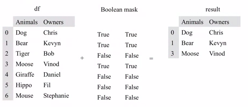
Boolean functions are created with the application of operators directly with panda strings or data frame objects.
To query, we can use the where function as in the NumPy library. The Where function uses the Boolean mask as a condition applied to DataFrame or Series and returns a new DataFrame or Series of corresponding shapes.
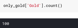
Let’s apply the Boolean function to our DataFrame data and create the National DataFrame for the gold medal at the Summer Olympics. First we will take out the countries with the gold medal, it.
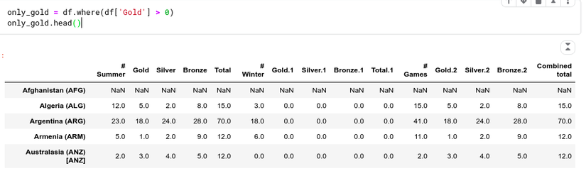
We see that only data from the countries that meet the conditions are retained. If all countries do not meet the conditions, write it as NaN. Most statistical vaults built in data frames ignore NaN values. For example, if we enter df.count () in the above data box, we will see 100 countries with gold medals awarded in the summer campaign, while if we count in the original data, we see There are a total of 147 countries.
Often we want to delete rows without data. To do this we can use the dropna() function. You can optionally provide removal of Na in the considered axes. Remember that the axes are only the orientation for the column or row and the default is 0, meaning the row.
1 2 3 | only_gold <span class="token operator">=</span> only_gold <span class="token punctuation">.</span> dropna <span class="token punctuation">(</span> <span class="token punctuation">)</span> only_gold <span class="token punctuation">.</span> head <span class="token punctuation">(</span> <span class="token punctuation">)</span> |
This is a bit verbose, below is a more concise example of how to query. You will see that there are no NaNs when you query this way, pandas automatically filters out rows with no values.
1 2 3 | only_gold <span class="token operator">=</span> df <span class="token punctuation">[</span> df <span class="token punctuation">[</span> <span class="token string">'Gold'</span> <span class="token punctuation">]</span> <span class="token operator">></span> <span class="token number">0</span> <span class="token punctuation">]</span> only_gold <span class="token punctuation">.</span> head <span class="token punctuation">(</span> <span class="token punctuation">)</span> |
We can also concatenate conditions by using or/and to create a complex query and the result is a simple Boolean. For example, we query the number of countries that won gold in one of the two Olympics.
1 2 | <span class="token builtin">len</span> <span class="token punctuation">(</span> df <span class="token punctuation">[</span> <span class="token punctuation">(</span> df <span class="token punctuation">[</span> <span class="token string">'Gold'</span> <span class="token punctuation">]</span> <span class="token operator">></span> <span class="token number">0</span> <span class="token punctuation">)</span> <span class="token operator">|</span> <span class="token punctuation">(</span> df <span class="token punctuation">[</span> <span class="token string">'Gold.1'</span> <span class="token punctuation">]</span> <span class="token operator">></span> <span class="token number">0</span> <span class="token punctuation">)</span> <span class="token punctuation">]</span> <span class="token punctuation">)</span> <span class="token comment"># kq:101</span> |
Or we want to query the number of countries with gold medals in both Olympics:
1 2 | <span class="token builtin">len</span> <span class="token punctuation">(</span> df <span class="token punctuation">[</span> <span class="token punctuation">(</span> df <span class="token punctuation">[</span> <span class="token string">'Gold.1'</span> <span class="token punctuation">]</span> <span class="token operator">></span> <span class="token number">0</span> <span class="token punctuation">)</span> <span class="token operator">&</span> <span class="token punctuation">(</span> df <span class="token punctuation">[</span> <span class="token string">'Gold'</span> <span class="token punctuation">]</span> <span class="token operator">></span> <span class="token number">0</span> <span class="token punctuation">)</span> <span class="token punctuation">]</span> <span class="token punctuation">)</span> <span class="token comment">#kq: 37</span> |
Another example for fun, which country has a gold medal at the winter Olympics but not yet at the summer Olympics. We do the following:
1 2 | df <span class="token punctuation">[</span> <span class="token punctuation">(</span> df <span class="token punctuation">[</span> <span class="token string">'Gold.1'</span> <span class="token punctuation">]</span> <span class="token operator">></span> <span class="token number">0</span> <span class="token punctuation">)</span> <span class="token operator">&</span> <span class="token punctuation">(</span> df <span class="token punctuation">[</span> <span class="token string">'Gold'</span> <span class="token punctuation">]</span> <span class="token operator">==</span> <span class="token number">0</span> <span class="token punctuation">)</span> <span class="token punctuation">]</span> |

Indexing Dataframes
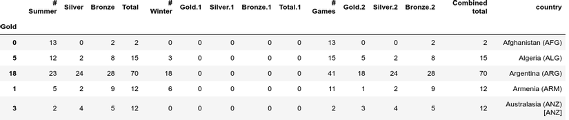
The index is needed for the item-level label and we know the rows correspond to the axis of 0. In the Olimpics data, we have set the index as the names of country names. We can set a column as an index column using the set_index function. The set_index function is a self-destruct process, it does not retain the current index. If you want to keep the current index, you need to create a new column and copy the values from the index attribute. Examples are as follows:
1 2 3 4 | df <span class="token punctuation">[</span> <span class="token string">'country'</span> <span class="token punctuation">]</span> <span class="token operator">=</span> df <span class="token punctuation">.</span> index df <span class="token operator">=</span> df <span class="token punctuation">.</span> set_index <span class="token punctuation">(</span> <span class="token string">'Gold'</span> <span class="token punctuation">)</span> df <span class="token punctuation">.</span> head <span class="token punctuation">(</span> <span class="token punctuation">)</span> |
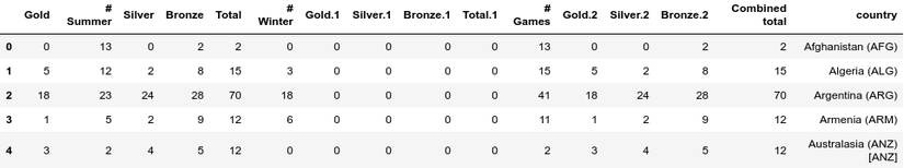
We can remove indexes created entirely by calling reset_index. This will create default index.
1 2 3 | df <span class="token operator">=</span> df <span class="token punctuation">.</span> reset_index <span class="token punctuation">(</span> <span class="token punctuation">)</span> df <span class="token punctuation">.</span> head <span class="token punctuation">(</span> <span class="token punctuation">)</span> |
Tl, dr
The article here is the longest, the longest post I have written so far. Thank you for reading. If you have any questions, you can leave a comment. See you at my next posts.