1. Introduction
If you have studied Computer Vision problems such as object detection and classification, you can see that most of the data in the image is displayed in great detail and detail in pixels. We just need to pass the model over networks like CNN and proceed to extract information. However, for data in the form of text, when the data information is not only contained in the form of pixels but also related semantics between words, how can we represent them? And Word Embedding is one of the ways we can display text data more efficiently.
2. What is Word Embedding?
Word Embedding is a vector space used to represent data that has the ability to describe relationships, semantic similarities, and context (context) of data. This space consists of many dimensions and words in that space that have the same context or semantics will be located close together. For example we have two sentences: “Today eat apple” and “Today eat mango”. When we do Word Embedding, “apple” and “mango” will be positioned close together in the space we represent because they are exactly the same position in a sentence.
3. Why do we need Word Embedding?
Let us try to compare with another representation that we usually use in multi-label problem, multi-task is one-hot encoding. If we used one-hot encoding , the data we would display would look like this:
| Document | Index | One-hot encoding |
|---|---|---|
| a | first | [1, 0, 0, …., 0] (9999 zeros) |
| b | 2 | [0, 1, 0, …., 0] |
| c | 3 | [0, 0, 1, …., 0] |
| …. | …… | …… |
| mom | 9999 | [0, 0, 0, …, 1, 0] |
| and so on | 10000 | [0, 0, 0, …., 0, 1] |
Looking at the table above, we see that there are 3 problems when we represent text as one-hot :
- Large computation cost: If the data has 100 words, the length of the one-hot vector is 100.If the data has 10000 words, the length of the one-hot vector is 10000. However, for the model to have high generality then In fact, the data can be up to millions of words, then the one-hot vector length will swell, making it difficult to calculate and store.
- Has little information value: The vectors are almost all zeros. And as you can see, for textual data the value contained in pixels (if input is an image) or other forms is very little. It is mainly located in relative position between words and related semantically. However, one-hot vector cannot represent that because it only indexes the input dictionary order, not the position of words in a particular context. To overcome that, the model often uses an RNN or LSTM class so that it can extract location information. There is another way, like in the transformer model, completely removing the word embeddig or RNN class and adding positional encoding and self-attention classes.
- Weak generality: For example we have three words that denote the mother: mother, cheek, bruise. However, the word bruising is relatively rare in Vietnamese. When performed with one-hot encoding, when it was put into model train, the bruise, although having the same meaning as the other two words, was classified into a different class due to different representations. If using word embedding, because it can display information about position, semantics, the word bruise will be close to the other two words. True to her embedding purpose
4. How to perform Word Embedding?
The two main methods used to calculate Word Embedding are the Count based method and the Predictive method . Both ways are based on the assumption that which words appear in the same context, a semantics will be positioned close together in the newly transformed space.
4.1. Count-based method
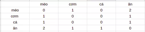
This method calculates the semantic relevance between words by statistically the number of co-occurrences of one word relative to other words. For example you have two sentences as follows:
Cats eat rice
Cats eat fish
==> We built a matrix of co-occurrences of the following words and found that rice and fish have similar meanings, so it will have close positions in the vector space.
However, this method has a disadvantage that when our data is large, some words have a large frequency but do not carry much information (as in English: a, an, the, … ) . And if we include this amount of data, the frequency of these words will obscure the value of words with more information but less common.
And to solve the problem, there is a solution that we re-weight the data to suit our problem. There is a very good algorithm used to solve this problem, which is TF_IDF transform . In which: TF is the frequency of occurrence of a word in data (term frequency) and IDF is a coefficient that helps reduce the weight of words that often appear in data (inverse document frequency). Thanks to the combination of TF vs IDF , this method can reduce the weight of words that appear a lot but do not have much information.
4.2. Predictive Methods (Word2Vec)
Unlike the Count-based method , the Predictive method calculates the semantic similarity between words to predict the next word by passing through a neural network with one or several layers based on the surrounding words input (context word ). A context word can be one or more words. For example, with the above two sentences, initially the two words rice and fish can be initialized quite far from each other, but to minimize loss between the two words and the context word (“Cat” and “eat”) , the position of The two words rice and fish in vector space must be close together. There are two common predictive methods :
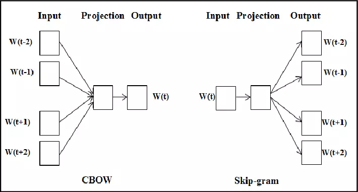
- Continuous Bag-of-Words (CBOW)
- Skip-gram
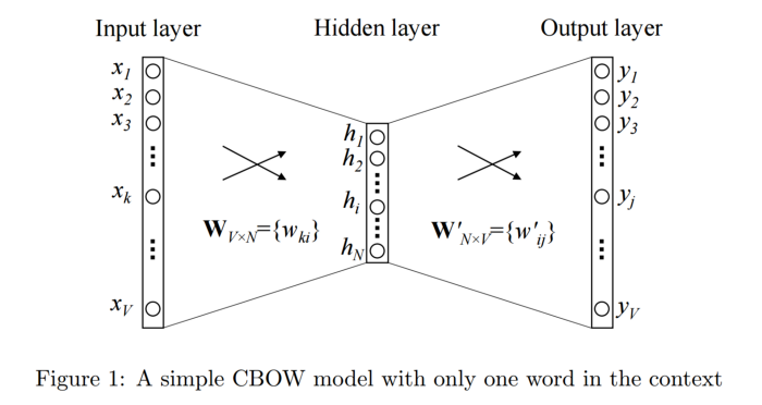
4.2.1. Continuous Bag-of-Words (CBOW)
CBOW model: This method takes input of one or more from context word and tries to predict output from the output (target word) through a simple neural layer. Thanks to the evaluation of output error with target word in one-hot form, the model can adjust the weight, learn the vector representation for target word. For example we have an English sentence like this: “I love you”. We have:
– Input context word: love
– Output target word: you
We transform the input context as one-hot passing through a hidden layer and doing softmax sorting to predict what the next word is.
4.2.2. Skip-gram
If CBOW uses input as context word and tries to predict the output word (target word), in contrast, the Skip-gram model uses target word input and tries to predict its neighbor words. They define the words as its neighbor (neightbor word) via the window size parameter. For example if you have a sentence like this: “I like to eat king crab “. And the initial input target word is the word crab . With the window size = 2, we will have neighbor words (like, eat, emperor, emperor). And we will have 4 input-output pairs as follows: (crab, like), (crab, king), (crab, sole), (crab, eat). The neightbor words are considered the same during training.
Summary : Comparing between the two methods Count based method and Word2Vec , when we train a large data set, the Count-based method needs relatively more memory than Word2Vec due to having to build a co-output matrix. show giant. However, since it is built on word statistics, when the amount of your data is large enough, you can train more data without worrying about increasing the size of the copper matrix that appears while increasing. model accuracy. Whereas it is completely impossible to increase the data when there is a relative amount of data to the Predictive method because the data is divided into train and valid sets. But in contrast, Word2Vec uses a machine learning model that increases the generality of the model while reducing computation and memory costs.
5. Conclusion
Recently, I have just started studying NLP, so the article may have many errors, confusing, so if something goes wrong, you can comment below the article. Thank you for watching my post.