We will start the 4th week of image processing, I learned image processing from the first term, now don’t remember much: v hours of re-reading and rewriting so I can remember.

We will recall our knowledge of the previous article including:The histogram is the histogram of the brightness division:

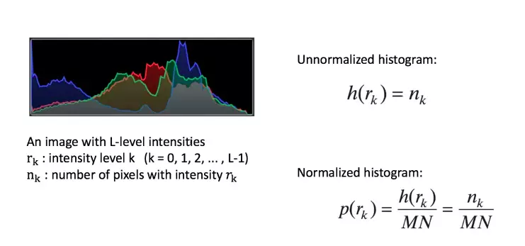
How does the histogram reflect the current state of the image? such as too dark, too bright, …

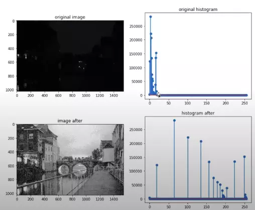
• Balance the gray level chart (Histogram Equalization)

As in previous articles, we are only interested in pixels, from this article onwards we will be interested in the pixels besides those pixels. In this article, we will explore filtering in pixel space. First of all we have some definitions.

Define

Neighbors of a pixel

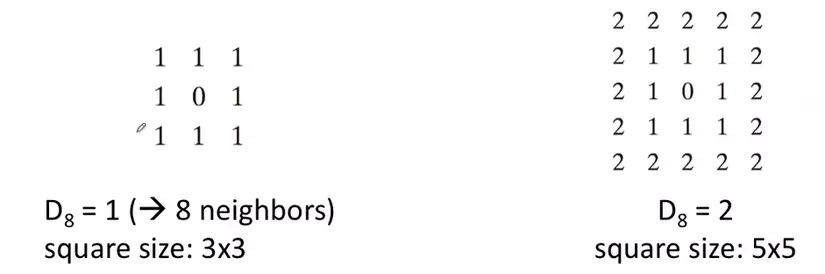
There are many definitions of neighboring pixels, most commonly 4 – neighbors, 8 – neighbors as shown below.

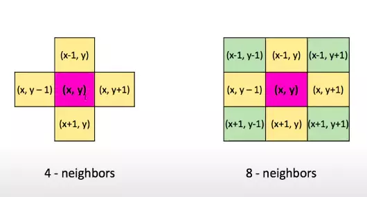
But what if we want to define the points closer to the point (x, y)? So, we have a new definition that is the distance between 2 pixels.

Distance between two pixels

We have 2 pixels p = (x, y) and y = (u, v)

The distance between 2 pixcel is using Euclidean formula:

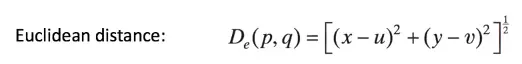
But the output may be a non-integer number, unusable in the definition of adjacent points. Therefore, we use the City-block formula, also known as the simpler Manhattan formula, resulting in an integer.

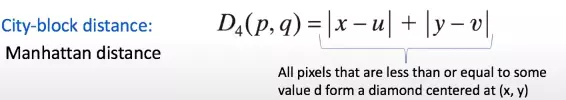
Apply having it in the definition of neighboring as follows:

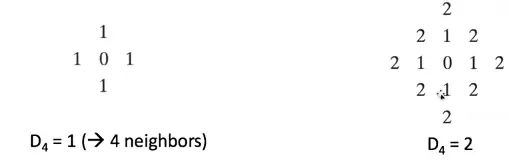
The difficulty of applying this formula is to represent the structure of these nearby points because it has a diamond shape. If performed, a matrix of squares or rectangles with lots of zeroes in the corners would be needed, and that would be a waste of resources. So we think of the new distance calculation formula.

Examples of definitions of points approaching this formula:

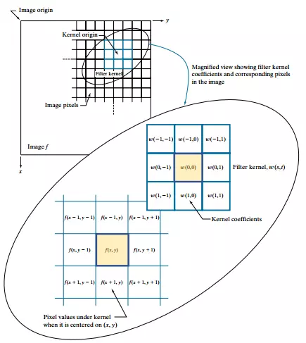
Spatical filter kernel

Or there are many other names: mask , template , window , filter , kernel . It is generally just a matrix whose size defines the proximity of the operation it applies and the value of each element represents the essence of the filter.

The spatical filter will change the image by replacing the value of each pixel by a function of the pixel and its neighbors.

Linear spatial filtering mechanism

Linear image transformation performs the calculation of the products between f image and kernel filter w and changes the pixel value to the total value found. Note that the position of the factor w (0,0) is the same as the position of the pixel f (x, y) in need of transformation.

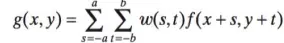
In general, transform an image f ( x , y ) f (x, y) $f(x,y)$ has dimensions $M$ $\ast$ $N$ $M\; *\; N$ M ∗ N uses a linear dimension kernel filter matrix $m$ $\ast$ $n$ $($ $m$ $=$ $2$ $a$ $+$ $first$ $,$ $n$ $=$ $2$ $b$ $+$ $first$ $)$ $m\; *\; n\; (m\; =\; 2a\; +\; 1,\; n\; =\; 2b\; +\; 1)$ m ∗ n ( m = 2 a + 1 , n = 2 b + 1 ) where a and b are negative numbers made by the formula:

As mentioned above, we have the calculation of the sum of products, in image processing, there are 2 operations that can do so. One operation is Correlation and the other is convolution . We will learn and distinguish it.

Correlation vs Convolution

Spatial correlation and convolution in 1D

With 1 dimension, the formula will become:

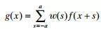
Here, for example, with a 1-D function: f f $f$ and a kernel w w $w$

The first thing we noticed was part of w w $w$ outside f f $f$ f f $f$ first × m 1 × m $1\times m$ $($ $m$ $–$ $first$ $)$ $/$ $2$ $(m\; –\; 1)\; /\; 2$ ( m – 1 ) / 2 numbers on either side of $f$ $f$ f to handle the start and end configurations of $w$ $w$ w for $f$ $f$ f . Figure (c) shows a correct pad function. Figure (c) shows that the center of the kernel must match the pixel we need to fix here and the first one.

Note that Zero padding is not the only padding option, we will discuss in more detail later in choosing padding

In the left image, Correlation is performed, while Convolution is different from Correlation in the first step, we will rotate the kernel. w w $w$ 180 degrees, the remaining steps to run sum the same product.

After doing the math, we also see that with Correlation , the function f f $f$ is reversed, but with Convolution , the output will be kept in the correct order.

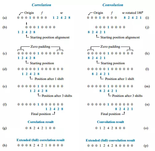
Spatial correlation and convolution in 2D

In 2D we have the same result.

Most of the image processing will be used as Convolution , but for convolutional neural network is called convolutional neural network with the operation called convolution but its nature is Correlation

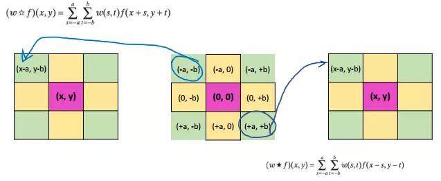
From the examples above, we have the mathematical formula for both:

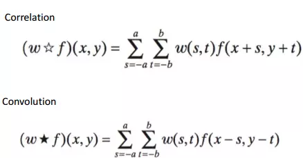
2 formulas only differ from the + sign above to the – sign below, the lower wallet below will help us better understand the formula:

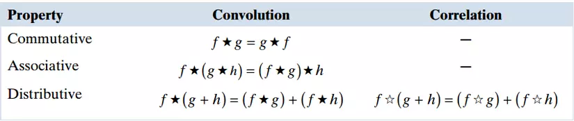
The basic properties of Convolution and Correlation are as follows:

Boundary issues

When we work with images working with convolution, an issue that arises when kernel g with image f then g will start to multiply with pixel at what value? There are 3 types as follows:

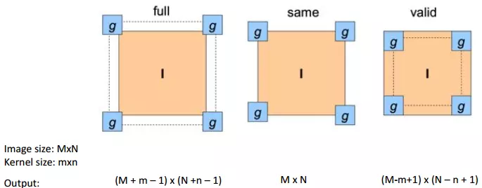
• Full type, the output of the image will be larger than the original image. The picture below describes the full type, below is the output image and below is the original image with padding as white cells.

• Similarly , the output of the image is the same size as the input image.

• Valid type, the output will be smaller than the input image.

What to do around the borders

In full and valid mode as above, we need to add padding. So how do we initialize the padding? Typically, there are types of initialization padding as follows:

• Pad a constant value (black). The example above we give the padding value 0 also known as zero-padding. In opencv use the command: cv2.BORDER_CONSTANT
• Wrap around (circulate the image): cv2.BORDER_WRAP
• Copy edge (copy the pixels at the edge). In opencv, use the command: cv2.BORDER_REPLICATE
• Reflect across edges (symmetrical). In opencv, use the command: cv2.BORDER_REFLECT

Spatial filter kernels

Filter design

Filter design is based on one of the following characteristics:

• Based on mathematical properties
  • Example 1: a filter that averages the pixels in the vicinity opens the image.
  • Example 2: A local derivative filter sharpens the image.
• Based on sampling a function in 2D space, the shape has the desired property
  • For example, take a sample from the Gaussian function to build a weighted average filter
• Based on frequency response (will study in Week Fourier Transform)

Smoothing Filters

• Used to reduce sharp conversion to intensity
  • Reduce extraneous details in the image (e.g. noise)
  • Smooth out the contours due to insufficient use of intensity levels in the image
• In this article, we will learn about the following kernels filters:
  • Mean filter / Box filter
  • Lowpass Gaussian filter
  • Order-statistic (nonlinear) filter

Mean filter / Box filter kernels

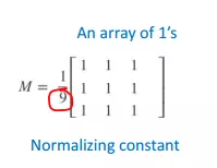
The idea behind the mean filter transformation method is simple. It is replacing the value of each pixel with the average of the neighboring pixels.

An mxn box filter is an array of size 1 mxn with the previous normalized constant of value 1 divided by the total value of the coefficients in the array (i.e. 1 / mn when all coefficients are 1 ). Below we have an example of a 3 x 3 box filter.

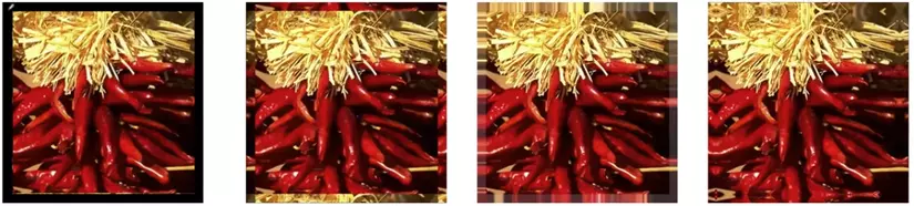
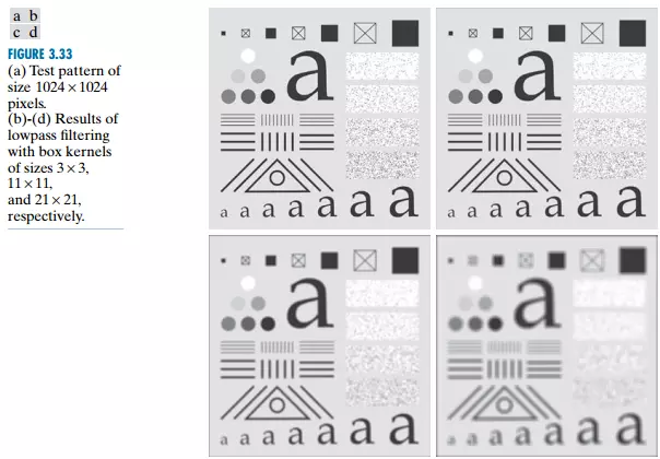
The kernel filter box is often used to smooth out lines or filter noise to enhance image quality. Below is an example when we apply the image a with the filter box size is 3 x 3, 11 x 11, 21 x 21 respectively. The more we see the increase in the size of the kernel, the more smooth and blurry the image go.

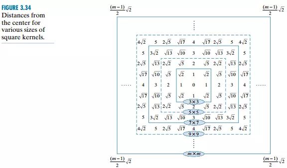
Gaussian Filter Kernels

The Gaussian filter kernels is similar to the box filter kernels but uses different matrices to represent the shape of the Gaussian function and it is used in the smoothing problem and has a better result than the box filter kernel.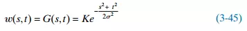

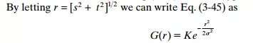
The value of r is the distance from the center to all the points in the function G. We can see the values ​​of r in the figure below.

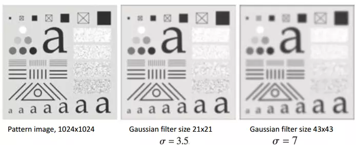
Some examples use Gaussian filters with different sizes and standard deviations with K = 1 in all cases.

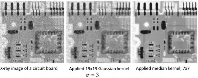
Comparison between box and Gaussian kernels

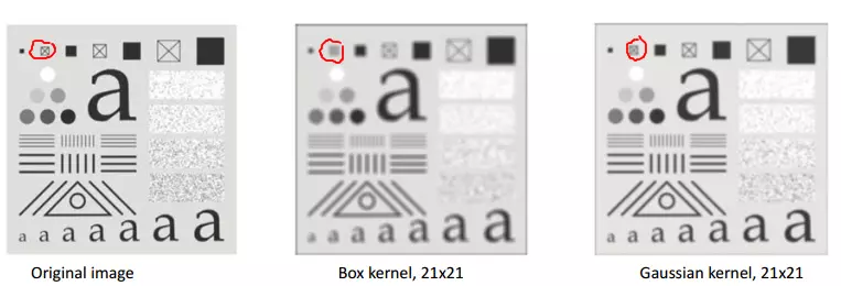
People who pay attention to the area of ​​their circle compartment will see that with the kernel of the same size, the kernel box will blur and change the shape of the image, while the Gaussian kernel will only blur. So in image processing, when you want to smooth the image people often use Gaussian kernel.

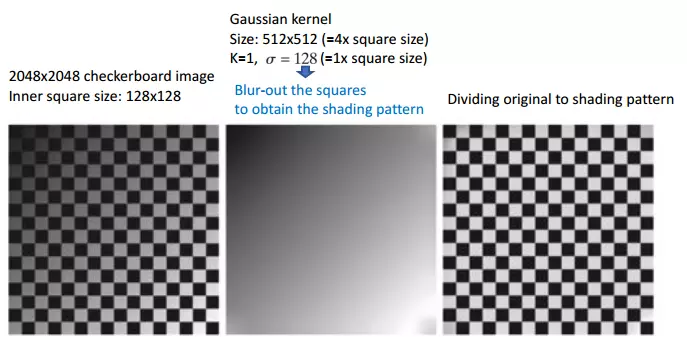
Another application of Gaussian filters is Shading correction. As the following example:

Order-statistic filters

This is a non-linear spatial filter, unlike the above filters that use addition and subtraction to divide, this filter is based on the order (rank) of pixels in the neighborhood and then replaces the value. of the central pixel is equal to the value determined by the ranking result.

The best known filters are Median filters, some of which are Max filters and Min filters.

Median filter

The Median filter replaces the value of the central pixel with the median of the intensity values ​​in its vicinity. It is great at reducing noise in situations such as random noise or salt-and-pepper noise.

Steps to make Median filter in 2D are as follows:

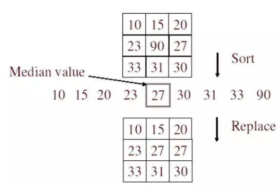
An example of the median filter applies to a salt-and-pepper noise image.

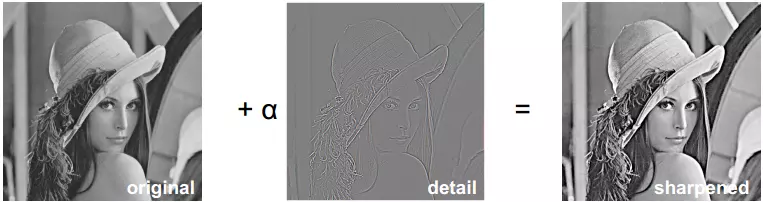
Unsharp masking

In this section, we will introduce the filter that sharpens the edges, the edge that can be interpreted as the transition from one brightness level to another. The steps taken to create unsharp masking will be as shown below.

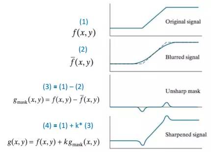
For k = 1, we call g (x, y) unsharp masking, with k> 1 will be called highbost filtering.

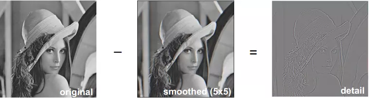
We have an example of unsharp masking to better understand the steps as follows:

summary

The article has been long here, if you have any questions or suggestions for your article to be better, please comment below. See you all in your next post.

References

1. Image processing – Le Thanh Ha
2. RC Gonzalez, RE Woods, “Digital Image Processing,” 4th edition, Pearson, 2018 Chapter 3.
3. Slide
4. Code github: here
5. http://deeplearning.net/software/theano/tutorial/conv_arithmetic.html
6. Week 4 – Spatial Filtering
7. https://docs.opencv.org/master/d2/de8/group__core__array.html