Introduce

Before Google published the article on Transformers ( Attention Is All You Need ), most of the natural language processing tasks, especially machine translation, used the Recurrent Neural Networks (RNNs) architecture. The weakness of this method is that it is very difficult to catch the deep dependence between the words in the sentence and the slow training speed due to the sequential input processing. Transformers was born to solve these 2 problems; and its variants like BERT, GPT-2 create new state-of-the-art for NLP related tasks. You can refer to the article BERT- a new breakthrough in technology of natural language processing of Google author Pham Huu Quang to understand more about BERT.

The Sequence-to-Sequence model uses RNNs

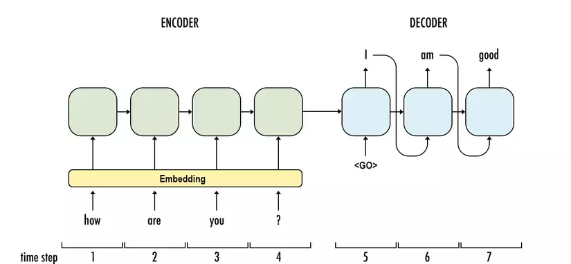
The Sequence-to-Sequence model accepts input as a sequence and returns output as a sequence. For example the Q&A problem, input is the question “how are you?” and the output is the “I am good” answer. The traditional method uses RNNs for both encoders (input encoders) and decoders (the decoding of inputs and the corresponding output). The first weakness of RNNs is that the train time is so slow, that people have to use the Truncated Backpropagation version to train it. However, the train speed is still very slow due to CPU usage, not taking advantage of parallel calculations on the GPU.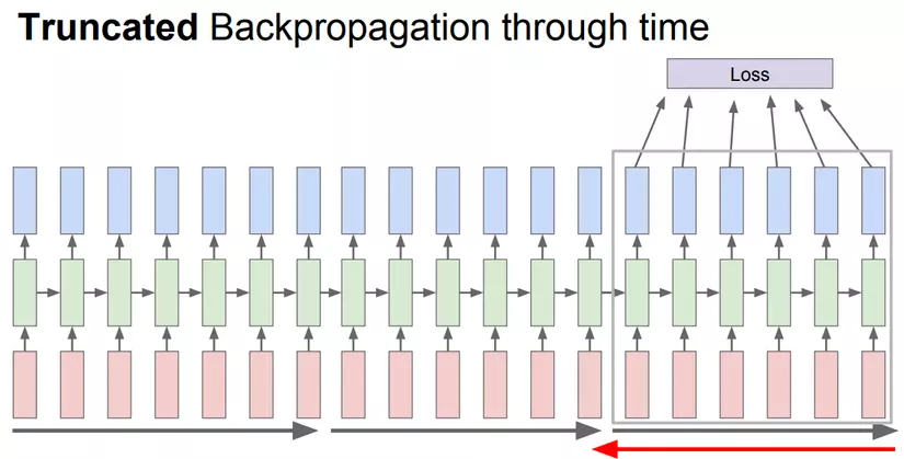

The second weakness is that it does not handle well with long sentences due to the phenomenon of Gradient Vanishing / Exploding. As the number of units gets bigger, gradients decrease in the final units due to the String derivative formula, resulting in a loss of information / dependency between units.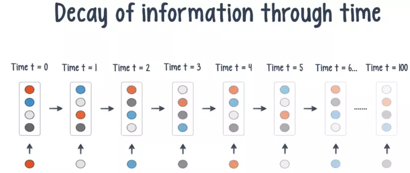

Launched in 1991, the Long-short Term Memory (LSTM) cell is a variant of RNNs that solves the problem of Gradient Vanishing on RNNs. LSTM cells have an extra C branch that allows all information to pass through the cell, helping to maintain information for long sentences.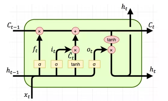

We seem to have solved the gradient vanishing problem, but LSTM is much more complex than RNNs, and obviously it also trains significantly slower than RNN.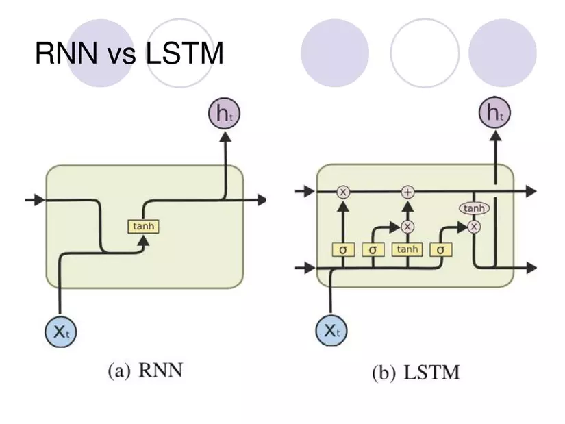

So is there a way to take advantage of the parallel computing power of the GPU to speed train for language models, while also addressing the weakness of long sentence processing? Transformers is the answer

Transformers

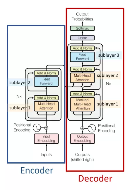
Transformers architecture also uses 2 parts Encoder and Decoder quite similar to RNNs. The difference is that the input is pushed at the same time . That’s right, at the same time; and there will be no more timestep concepts in Transformers. So which mechanism has replaced the “recurrent” of RNNs? That’s Self-Attention , and that’s why the paper name is “Attention Is All You Need” (fun fact: This name is after the movie “Love is all you need” ). Now let’s go into each component one by one

Encoder

1. Input Embedding

Computers cannot understand words but only read numbers, vectors, and matrices; so we have to represent the sentence in vector form, called input embedding. This ensures that the words near the meaning have the same vector. There are already quite a lot of pretrained word embeddings like GloVe, Fasttext, gensim Word2Vec, … for you to choose.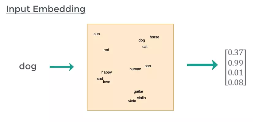

2. Positional Encoding

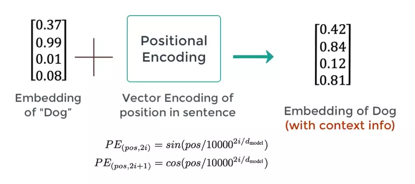
Word embeddings partly help us to represent the semantics of a word, but the same word in different positions of the sentence has different meanings. That’s why Transformers has a Positional Encoding section to inject more information about the position of a word

P E ( p o S , 2 i ) = sine ⁡ ( p o S / 1000 0 2 i / d m o d e l ) P E ( p o S , 2 i + first ) = cos ⁡ ( p o S / 1000 0 2 i / d m o d e l ) begin {aligned} P E _ {(pos, 2 i)} & = sin left (pos / 10000 ^ {2 i / d _ { mathrm {model}}} right) \ P E _ {(pos, 2 i + 1)} & = cos left (pos / 10000 ^ {2 i / d _ { mathrm {model}}} right) end {aligned} P E (p o s, 2 i) P E (p o s, 2 i + 1) = Sin (p o s / 1 0 0 0 0 2 i / d m o d e l ) = cos ( p o s / 1 0 0 0 0 2 i / d m o d e l )

Inside p o S pos $pos$ is the position of the word in the sentence, PE is the value of the th element i i $i$ d m o d e l d _ { mathrm {model}} d m o d e l . Then we add PE vector and Embedding vector:

3. Self-Attention

Self-Attention is a mechanism that helps Transformers “understand” the relationship between words in a sentence. For example, how does the word “kicked” in the “I kicked the ball” sentence relate to other words? Obviously it is closely related to the word “I” (subject), “kicked” is itself up will always “strongly related” and “ball” (predicate). In addition, the word “the” is a preposition so the association with the word “kicked” is almost absent. So how does Self-Attention extract these “relevance”?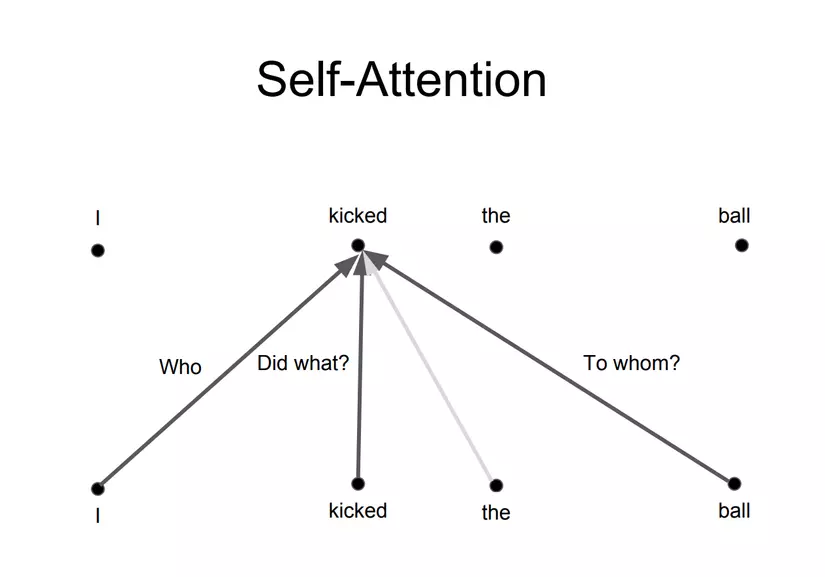

Returning to the overall architecture above, you can see that the input of the Multi-head Attention module (Self-Attention essentially) has 3 arrows, which are 3 vectors Querys (Q), Keys ( K) and Values ​​(V). From these 3 vectors, we will calculate attention Z vector for a word according to the following formula:

Z = softmax ⁡ ( Q ⋅ K T D i m e n S i o n o f v e c t o r Q , K or V ) ⋅ V Z = operatorname {softmax} left ( frac {Q cdot K ^ {T}} { sqrt {D imension ~ of ~ vector ~} Q, K text {or} V} right) cdot V Z = s o f t m a x ( D i m e n s i o n   o f   v e c t o r   Q , K or V Q ⋅ K T ) ⋅ V

The formula is quite simple, it is done as follows. First, to get 3 vectors Q, K, V, input embeddings is multiplied by 3 corresponding weight matrices (tuned during training) WQ, WK, WV.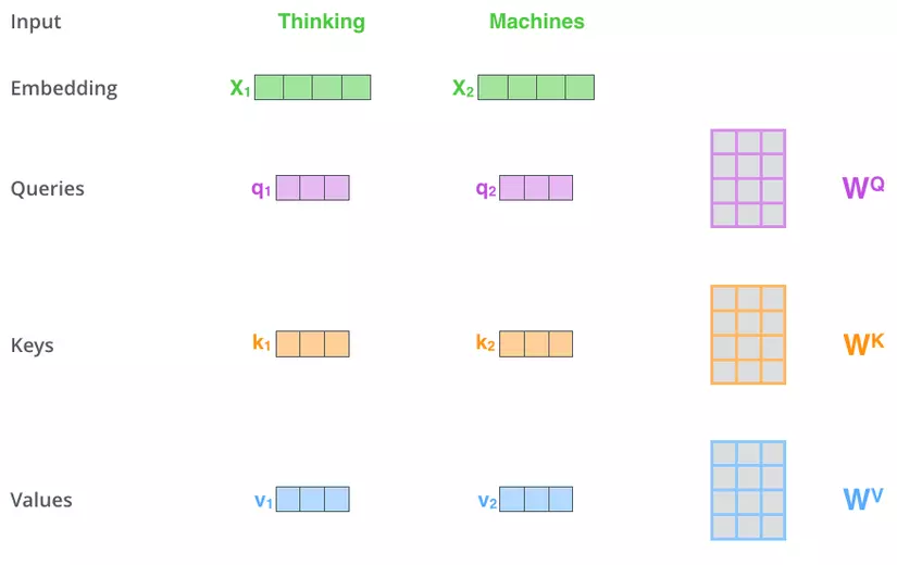

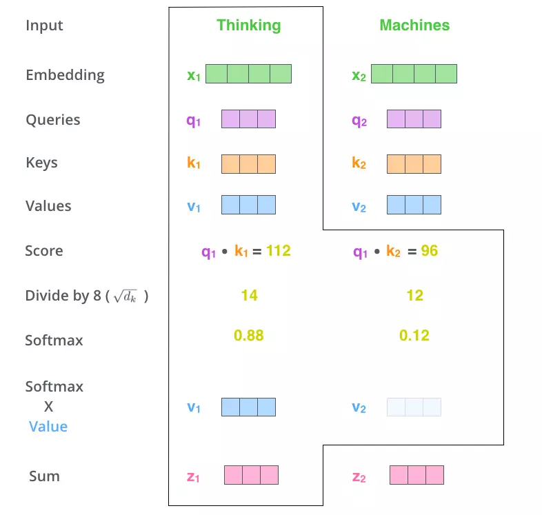
At this point, the vector K acts as a key to represent the word, and Q will query the vector K of the words in the sentence by multiplying with these vectors. The purpose of convolution is to calculate the relationship between words. Accordingly, two words related to each other will have a large “Score” and vice versa.

The second step is the “Scale” step, which simply divides “Score” by the square root of the number of dimensions of Q / K / V (in the figure 8 divided by Q / K / V is 64-D vectors). This helps keep the “Score” value independent of the length of the Q / K / V vector

The third step is softmax the previous results to achieve a probability distribution on the words.

In the fourth step we multiply that probability distribution by vector V to eliminate unnecessary words (small probability) and retain important words (large probability).

In the final step, the vectors V (multiplied by the softmax output) add up, creating the vector attention Z for a word. Repeat the above process for all words we get the attention matrix for 1 sentence.

4. Multi-head Attention

The problem with Self-attention is that the attention of a word will always “pay attention” to itself. This makes sense, because “it” is clearly related to “it” the most . For example:

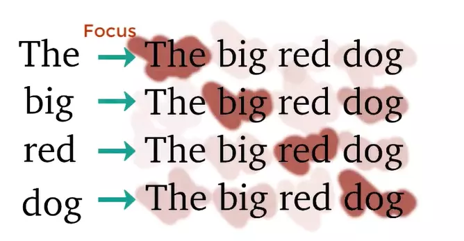
But we don’t want this, what we want is the interaction between DIFFERENT words in the sentence. The author has introduced a more upgraded version of Self-attention called Multi-head attention. The idea is very simple, instead of using 1 Self-attention (1 head), we use many different Attention (multi-head) and maybe every Attention will pay attention to a different part of the sentence.

Because each “head” will produce a separate attention matrix, we have to concatenate these matrices and multiply by the WO weight matrix to produce a unique attention matrix (weighted sum). And of course, this weight matrix is ​​also tuned during training.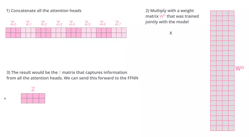

5. Residuals

As you can see in the overview model above, each sub-layer is a residual block. Like residual blocks in Computer Vision, skip connections in Transformers allow information to pass through sub-layers directly. This information (x) is added to its attention (z) and performs Layer Normalization.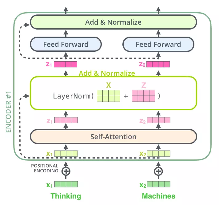

6. Feed Forward

After being Normalized, the vectors z z $z$ is sent over a fully connected network before pushing through the Decoder. Because these vectors are not dependent on each other, we can take advantage of parallel calculations for the whole sentence.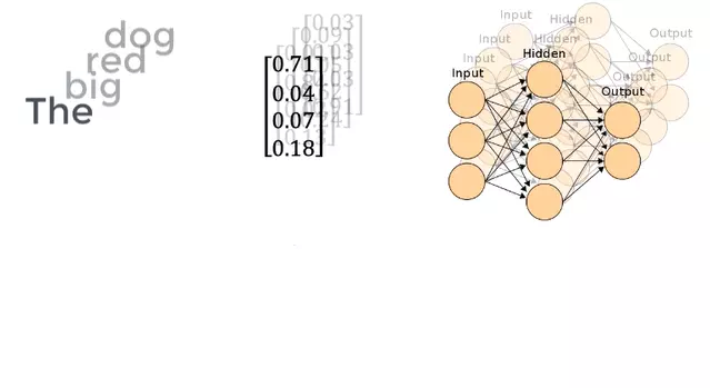

Decoder

1. Masked Multi-head Attention

Suppose you want Transformers to perform the English-France translation problem, then Decoder’s job is to decode information from the Encoder and generate each French word based on THAT WORDS. So, if we use Multi-head attention on the whole sentence as in Encoder, Decoder will “see” the next word that it needs to translate. To prevent that, when the Decoder translates from th i i $i$ , the back of the French sentence will be masked and Decoder is only allowed to “see” the part it has translated earlier.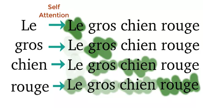

2. The decode process

The decode process is basically the same as the encode, except that Decoder decode word by word and the input of Decoder (French sentence) is masked. After the masked input passes through Decoder’s sub-layer # 1, it will not multiply by 3 weight matrices to create Q, K, V any more but only multiply by 1 WQ weight matrix. K and V are taken from Encoder with Q from Masked multi-head attention put into sub-layer # 2 and # 3 similar to Encoder. Finally, the vectors are pushed into the Linear layer (which is a Fully Connected network) followed by Softmax to give the probability of the next word.

The following two pictures visually depict the process of Transformers encode and decode

Encoding :

Decoding :

Conclude

Above I have introduced to you about the Transformers model – a model that I find very good and worth to learn. Now Transformers, its variants, along with pretrained models have been integrated in many packages that support tensorflow, keras and pytorch. However, if you want to implement from the beginning, you can refer to detailed instructions Transformer model for language understanding of tensorflow.

References:

[1] The Illustrated Transformer

[2] Transformer Neural Networks – EXPLAINED! (Attention is all you need)