The basic sort algorithm

1. the Concept

Sorting problem is the problem of solving the organization of data in a certain order, usually ascending or descending.

Summary of ascending sort problem:

Input: An array of n elements A = (

a first , a 2 , a 3 , . . . , a n a_1, a_2, a_3, …, a_n$a^1,A^2,A^3,...,A^n$ )

Output: A permutation of A is array A ‘= (

a first ′ , a 2 ′ , a 3 ′ , . . . , a n ′ a’_1, a’_2, a’_3, …, a’_n$a^1,A^2,A^3,...,A^n$ ), meeting the following conditions:

a first ′ < = a 2 ′ < = a 3 ′ < = . . . < = a n ′ a’_1 <= a’_2 <= a’_3 <= … <= a’_n${}^1$

2 basic maths for sorting problems:

1. Swap operation: Is a 2-variable value inversion

2. Comparative operation: Returns true if a> b and returns false for otherwise.

These are 2 sub operations that are often used in sort problems. Like the +- magic in arithmetic.

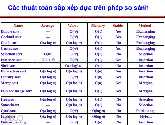
2. Three basic sort algorithms

2.1. Insertion Sort

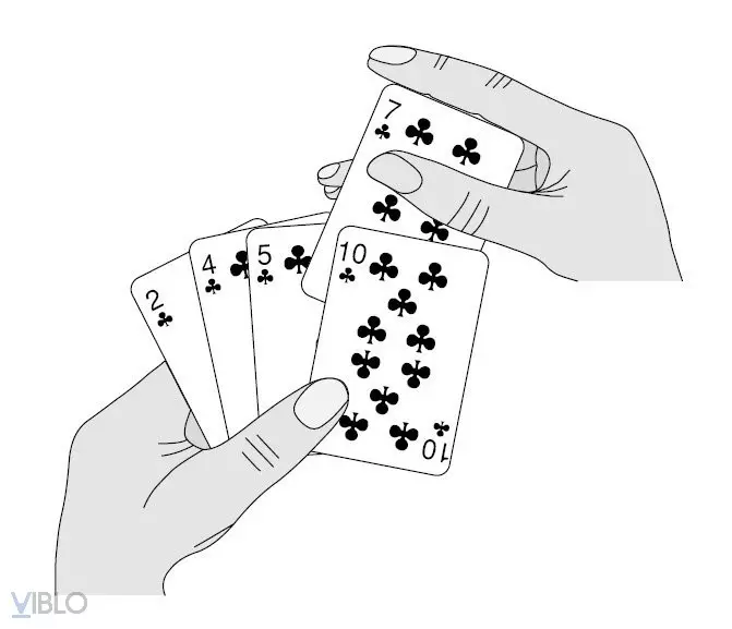
The idea: Insertion Sort takes its ideas from chơi bài , based on how the player “inserts” a new card into the hand that has been laid out.

Algorithm:

• At steps k = 1, 2, …, n puts the kth element in the given array in the correct position in the sequence of the first k elements.
• The result is that after the kth step, there will be the first k elements in order.

For example: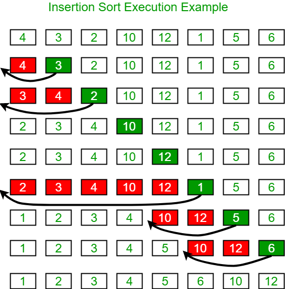

Evaluate:

• Best Case: 0 swap, n-1 compare (when input sequence is already sorted)
• Worst Case:
  n 2 n_2$n^2$ / 2 swap and compare (when the input sequence is in the opposite order to the order)
• Average Case:
  n 2 n_2$n^2$ / 4 swap and compare

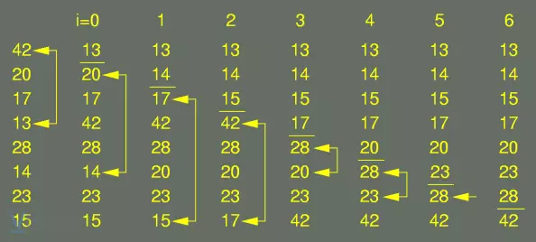
2.2. Sort selection

The idea of ​​Selection sort is to find each element for each position of the permutation array A ‘to be searched.

Algorithm:

• Finds the smallest element in position 1
• Finds the next smaller element in position 2
• Finds the next smaller element in position 3
• …

For example: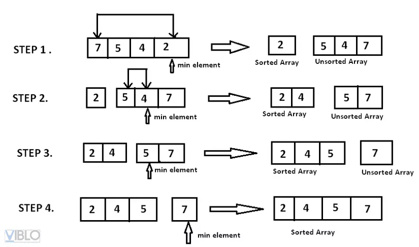

Evaluate:

• Best case: 0 swap (n-1 as in the code),
  n 2 n_2$n^2$ / 2 comparison.
• Worst case: n – 1 swapped and
  n 2 n_2$n^2$ / 2 comparison.
• Average case: O (n) swaps and
  n 2 n_2$n^2$ / 2 comparison.

2.3. Bubble Sort

The idea: Bubble Sort, as the name implies, is the algorithm that pushes the largest element to the end of the sequence, and the smaller value elements will gradually move to the beginning of the sequence. Like bubbles, lighter elements will float above and vice versa, larger particles will sink.

Algorithm: Browse the array from the first element. We will compare each element with the element immediately preceding it, if they are in the wrong position, we will swap places with each other. This process will be stopped if you encounter a browse from the beginning of the sequence to the end of the sequence without having to change any two parts of the word (ie all the elements have been arranged in the right position).

For example: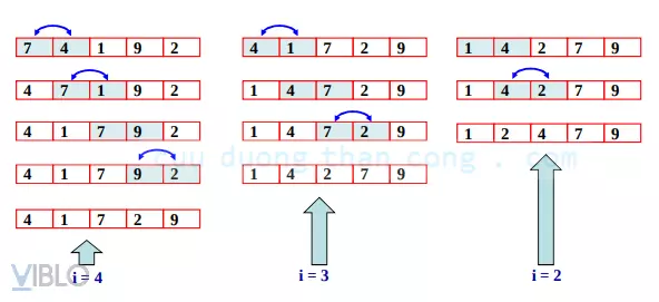

Evaluation: Simple but Bubble is the least efficient of the 3 algorithms in this section

• Best case: 0 swaps,
  n 2 n_2$n^2$ / 2 comparison.
• Worst case:
  n 2 n_2$n^2$ / 2 switch and compare.
• Average case:
  n 2 n_2$n^2$ / 4 change seats and

  $n$ $2$ $n\_2$n 2 / 2 comparison.

Compare 3 algorithms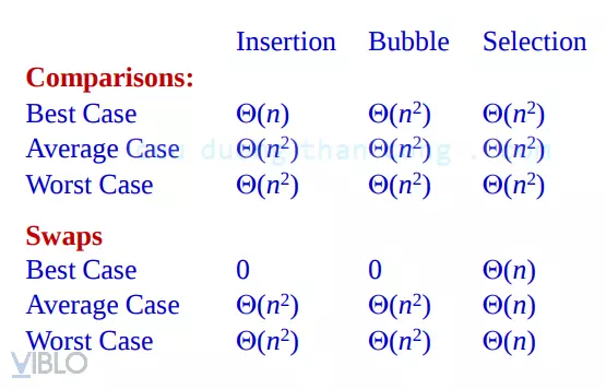

3. Merge Sort

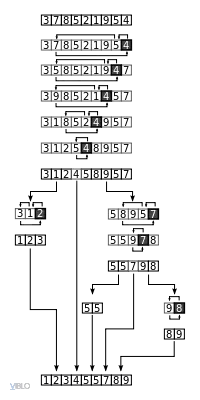
The merge sort is a comparative sort algorithm. This algorithm is a relatively typical example of John von Neumann’s division and rule algorithm:

• Divide (Divide): Divide the sequence of n elements to be arranged into 2 sequences, each sequence has n / 2 elements.
• Tri (Conquer): Arrange each sub-sequence recursively using a mix sort. When the sequence has only one element left, return this element.
• Combine: Combine two merged child sequences to get the sorted sequence of all elements of both sub sequences.

Algorithm:

Mixing algorithm :

Suppose there are two sequences sorted L [1 ..

n first n_1$n^1$ ] and R [1 ..

n 2 n_2$n^2$ ] . We can mix them into a new sequence M [1 ..

n first + n 2 n_1 + n_2$n^1+n^2$ ] organized in the following way:

• Compare the two leading elements of the two arrays, taking the smaller element into the new sequence. Continue this way until one of the rows is empty.
• When either sequence is empty, we take the remainder of the other sequence at the end of the new sequence.

When that happens, we will obtain the range we are looking for.

Rating: O (n * logn)

For example: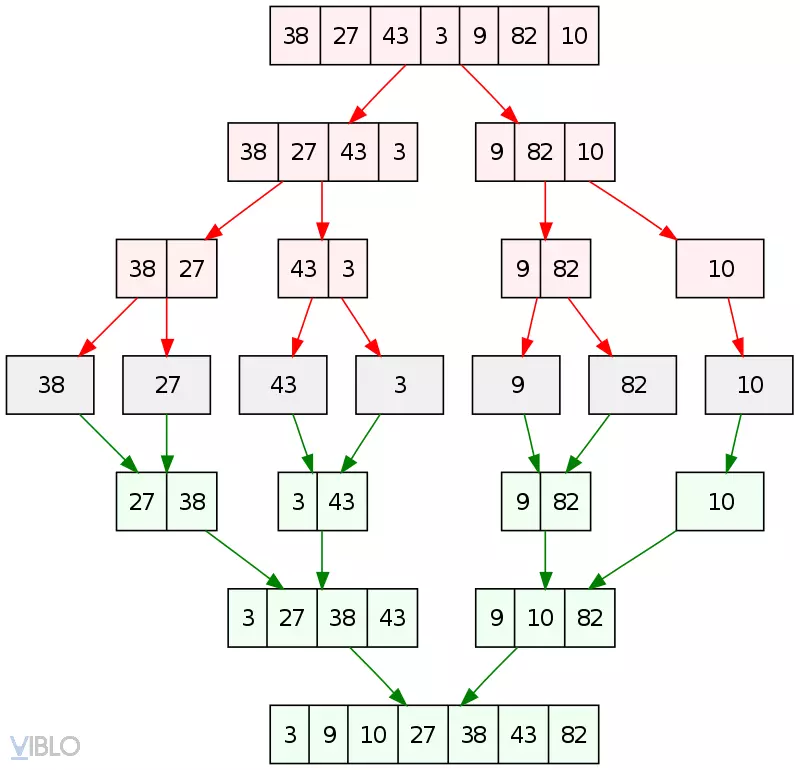

4. Quick Sort

Quick Sort (QS) was developed by Hoare in 1960. According to statistics, QS is the fastest sorting algorithm available today.

QS has an average time of O (n * log n), but its worst time is O (n * log n).

n 2 n_2$n^2$ ).

Similar to Merge sort, Quick sort is a sorting algorithm developed based on division and value technique:

1. Base recursive anchor. If the sequence has only one element left, it is the sorted array and returns this sequence without doing anything.
2. Divide (Divide):
   • Select an element in the sequence and call it a p (pivot) element.
   • Divide the given sequence into two sub sequences: The left sub-sequence ( L ) consists of elements no bigger than the latch element, and the right sub-sequence ( R ) consists of elements no less than the latch element. This operation is called manipulation Phân đoạn (Partition).
3. Tri (Conquer): Recursive algorithm recursively for two sub-rows L and R.
4. Combine: The sequence is arranged as L p R.

Algorithm:

Select latch element :

Selecting the key element is crucial to the performance of the algorithm. It is best to select the latch element as the median of the list. However, this way is very difficult, so we can choose key elements in the following ways:

• Select the top or bottom element as a latch element.
• Select the element in the middle of the range as a key element.
• Select the median element in the top 3, middle and last position as a latching element.
• Selects random element as a key element. (This may result in the possibility of special circumstances.)

Partition Segment Algorithm : The purpose of the Partition(A, left, right) function Partition(A, left, right) is to divide A [left..right] into two segments A [left..pivot –1] and * A [pivot + 1..right] , such that:

• A [left..pivot –1] is a collection of elements with value less than or equal to A [pivot] .
• A [pivot + 1..right] is a collection of elements with a value greater than A [pivot] .

Example of QS: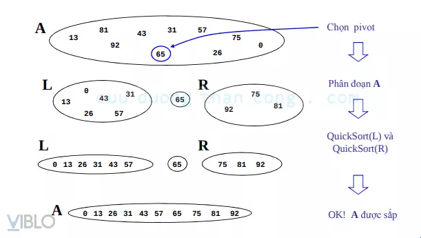

Evaluation: Quick-Sort calculation time depends on whether the segmentation is balanced or unbalanced, and this depends on the selection of the latch element.

• Unbalanced segment: O (
  n 2 n_2$n^2$ )
• Perfect segment: O (n * logn)

5. Heap Sort

Definition * Heap (heap) is a nearly complete binary tree with two properties: – Structural property: all levels are full child nodes, except the last level. The last level is filled from left to right. – Ordered or heap property: For each node x, there is Parent (x) ≥ x .

Representing the stack as an array, we have:

• The root of the tree is A [1]
• The left child of A [i] is A [2 i] *
• The right child of A [i] is A [2 i + 1] *
• A [i] ‘s father is A [i / 2]
• The heap number of elements is Heapsize [A] ≤ length [A]

Classification: There are 2 types

• Max-heaps: for every node i, except root: A [parent (i)] ≥ A [i]
• Min-heaps: for every node i, except root: A [parent (i)] ≤ A [i]

We will consider the problem with max-heap, min-heap similar.

Calculation of max-heap property (Back to the pile)

Consider the problem:

Suppose there is an i node with a value smaller than its child, and the left subtree and right subtree of i are max-heaps

Recursive algorithm:

• Swap i with the older one
• Move down under the tree
• Continue the process until node i is no longer younger than the child.

For example: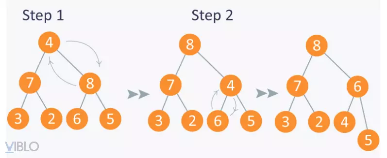

Heapsort algorithm

The idea: With A being a max-heap, if each sub-tree has a parent node from 1 to n / 2 being max-heaps, then A is a descending array.

For example:

Above are some of the sorting algorithms I have learned, if there is anything wrong, you can give me suggestions.

Hope this article is helpful to you. See you in the next posts.

References:

Data structures and algorithms – Nguyen Duc Nghia, Hanoi University of Science and Technology Publishing House, 2013

Mergesort

Quicksort

Heap sort