Continuing part I would like to introduce to you 10 more tips from Google Sheet offline.
11. Drag data from other Google Sheets
- Use the IMPORTRANGE function
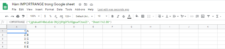
- Formula: = IMPORTRANGE (“spreadsheet_URL”, “Sheet and cell references”)
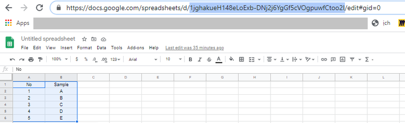
- Examples: = IMPORTRANGE (“1jghakueH148eLoExb-DNj2j6YgGf5cVOgpuwfCtoo2I”, “Sheet1! A2: B6”)
spreadsheet_URL:
Sheet and cell references: are the sheet and from & to of the value cell we want to get the result.
Result:
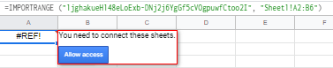
Note: there will be a small popup showing out asking us to connect to the sheet that we want to get data from. You just need to select Access allow , the data of that sheet will be transferred to the current sheet according to the formula.
12. Lock cells to prevent unwanted changes
– Purpose: want to limit editing rights of members sharing files. – How to lock: Step 1: Highlight the area you want to lock. Step 2: On the toolbar, select Data> Protected sheets and ranges 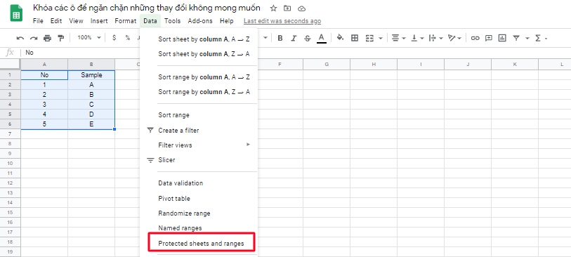
Step 3: The Protect Sheets and Ranges options bar will appear on the right side of the window. Here, you can enter a brief description of the reason for the key in the Enter a description box 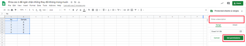
Step 4: Click the green “Set Permissions” button to switch to the set permissions for locked cells.
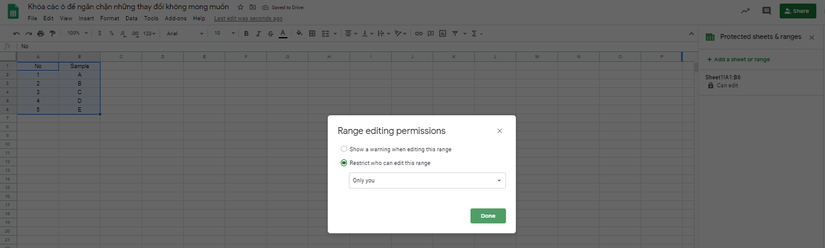
Step 5: After setting up permissions is complete, click Done. If you want to show warning when others edit, then check the Show a warning when editing this range
13. Convert files to Sheets
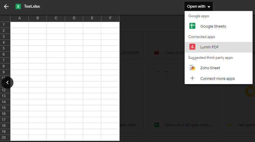
– How to transfer: Step 1: Upload the .XLSX file to google drive Step 2: Open the .XLSX file using Google sheets
** Step 3: ** on the toolbar select File> Save as Google Sheets
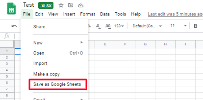
Step 4: After clicking Save as Google Sheets will generate a new file similar to the Google Sheets format and you can delete the old .XLSX file format.
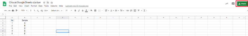
14. Share your Google Sheet
– How to share:
Step 1: Click the green Share button on the right corner of the screen
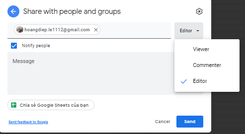
Step 2: Input the email addresses you want to share.

Step 3: Select the permission for the account you want to share and then click Done.
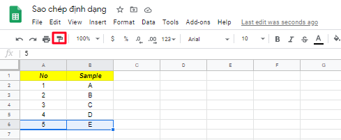
15. Copy format
- Use the Format Painter to format cells and use a similar style in other cells.
- Steps to be followed:
Step 1: Select the cells that you want to copy the format from.
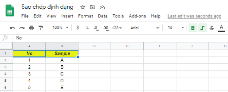
Step 2: Click on the format painter and drag over the cells that you want to apply the formats to.
16. Enter from Form into Sheets
Step 1: In the toolbar of Google spread sheets select Insert > Form
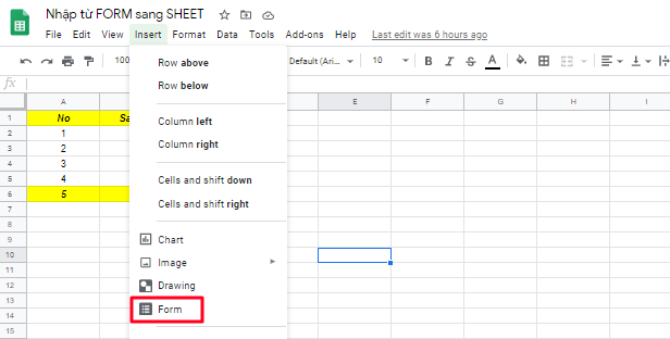
Step 2: The interface will appear as follows and here you can create a custom form.

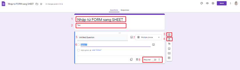
Explanation of items: 1: title of the form (this title will default to be taken by the title of google sheet) 2: description of form 3: add question 4: import form 5: place to input question 6: place to input answer 7: question answer method 8: establish whether the answer is required or not? If the answer is required then turn this function on
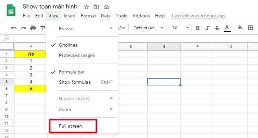
17. Show full screen
– Purpose: to help limit distractions appearing on the computer screen. – How to show full screen: press View > Full screen
18. Conditional Formatting
Purpose: conditional formatting is used for large spreadsheets, using a coloring tool to help you view large amounts of data easily to handle it
How to perform conditional formatting:
Step 1: On the toolbar select Format > conditional formatting
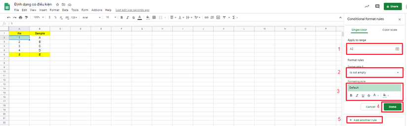
Step 2: Then on the right, Conditional format rules will appear on the screen to set conditions for data.

Explanation of items:
1: the cell for which you want to set the condition
2: spot setting condition. The conditions are as follows:
| English | Vietnamese |
|---|---|
| Cell is empty | Empty box |
| Cell is not empty | The cell is not empty |
| Text contains | Contains text |
| Text does not contain | Does not contain text |
| Text is exactly | Have exact same text |
| Date is | Contains the date |
| Date if before | Contains the previous date … |
| Date is after | Contains the following date …. |
| Greater than | Bigger… |
| Greater than or equal to | Greater than or equal |
| Less than | Less… |
| Less than or equal to | Less than or equal |
| Is equal to | Equal to … |
| Is not equal to | Not equal to … |
| Is not between | Not in the middle … |
| Custom Formula | According to the formula |
3: color setting for the condition
4: press Done to complete the condition setting
5: add another condition
19. Freeze / freeze rows / columns in Google sheets
-Purpose: fixing a row or column is the hardening of that row / column at the top of the worksheet, whether you scroll down or drag the article sideways, the row / column remains in this position.
-How to freeze rows / columns:
Step 1: Open the Google Sheets page, click the cursor on the number or word of that row / column.
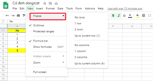
Step 2: Select View > Freeze , then you will see a menu of options appear. In this options table you will be able to select the row / column that you want to fix.
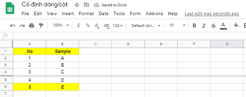
Step 3: As a result, the row or column you select has been frozen and fixed with a gray border to separate the rest area, and cannot be moved no matter where you drag the mouse. again.
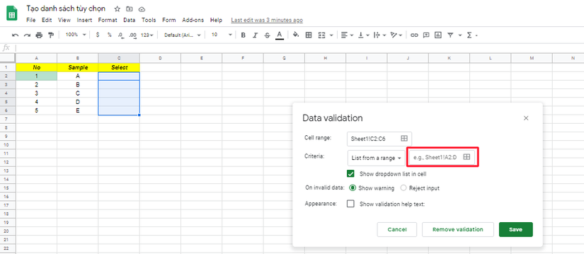
20. How to create an option list
– How to create a dropdown menu:
Step 1: Select the cell where you want to create the dropdown list
Step 2: Next, choose Data > Data validation
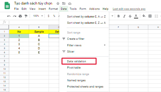
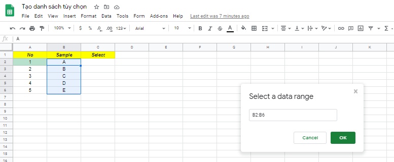
Step 3: Then it will show popup with title Data validation as below and you can set the drop-down list by clicking on the red box.
Step 4: After clicking the red box, a popup will appear again with the title Select a data range and you will select the range of options you want> click OK > click Save as the setting is complete.