1. Image stitching algorithm
1.1 Introduce
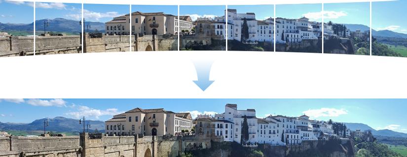
Surely everyone has ever seen or used the panorama photography function of Smart phones. These panorama photos are quite large in size, wide view and with smart phones, we can create by panning the camera slowly over the scene to capture. The applications of this problem class are many. In the past, when the quality and the width of the camera view was limited, people had to use these algorithms to create high-resolution images with panoramic views. Or as the photo below that caused fever in 2019, showed by the neighbors Tung Cua is a 24.9 billion pixel photo taken from “Satellites with quantum technology”, which can be zoomed to every street corner, window or child. people in Shanghai. This photo was later discovered that it was actually just a photo made up of tens of thousands of photos created by Jingkun Technology . So what is the algorithm / technology behind these magical panoramas, I will write about it today.
This topic is called Image Stitching or Photo Stitching , combine – combine a set of pictures to make a large image, these sub-images have overlapping areas. Previously, people followed the ” directly minimizing pixel-to-pixel dissimilarities ” method, which means finding overlap by matching 2 regions of 2 images with the smallest difference. However, this approach proved ineffective. Then, the Feature-based solution was born. Below is a Flow for the Image Stitching problem in Feature-base direction.
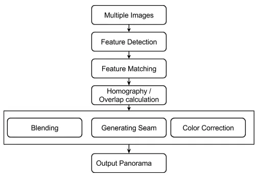
This is a simple flow for newbies, in this article I will present with the case of only 2 images:
- Use specialized algorithms to detect a set of keypoints for each image. These keypoints are special, characteristic and not affected (or slightly affected) by brightness, rotation, scale (zoom) …
- Find a way to match these 2 keypoint sets, find the corresponding keypoint pairs.
- Based on those keypoint pairs to find out how to transform (transform) -> to combine 2 images together. Thus obtained panorama image.
Note It sounds very simple, right. In fact, we still have to deal with the difference in brightness between two images or blurred outlines, colors …. To simplify the content of this article, I will not write about post-processing steps. there.
1.2 Key points detection
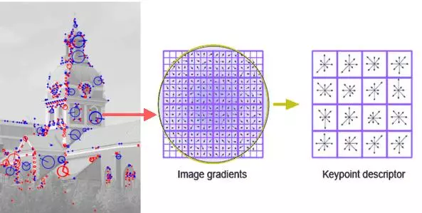
If you have been exposed to image processing problems, you will be familiar with using Feature extractors such as SIFT, SUFT, ORB … Opening the class of these algorithms is SIFT – Scale Invariant Feature Transform. SIFT is used to detect keypoints in an image. These keypoints are distinctive, feature-rich and distinctive. For each Keypoint, SIFT returns the coordinates (x, y) with a Descriptor – a 128- dimensional vector representing the features of that keypoint.
These vector descriptor are not / less affected by rotation, light, scale … That means that the same point appearing on 2 images (regardless of shooting angle, different brightness) will have approximately the same descriptor. Figure H1.3 illustrates that.
In opencv provides a full range of Keypoint Extractor SIFT, SUFT, ORB … The code is quite simple:
1 2 3 | sift <span class="token operator">=</span> cv2 <span class="token punctuation">.</span> xfeatures2d <span class="token punctuation">.</span> SIFT_create <span class="token punctuation">(</span> <span class="token punctuation">)</span> kp <span class="token punctuation">,</span> des <span class="token operator">=</span> sift <span class="token punctuation">.</span> detectAndCompute <span class="token punctuation">(</span> img <span class="token punctuation">,</span> <span class="token boolean">None</span> <span class="token punctuation">)</span> |
Note: SIFT is copyrighted. If used for commercial purposes, it is necessary to pay fees or with the consent of the author.
1.3 Key points maching
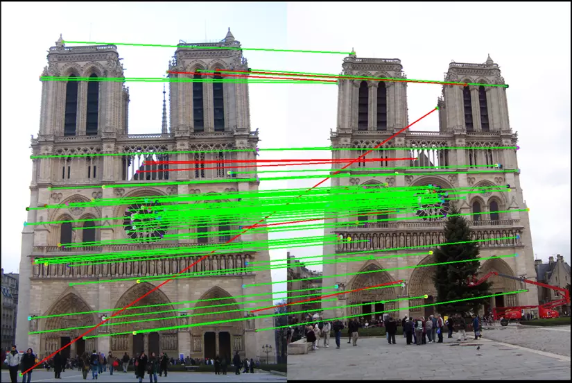
Suppose we have extracted 2 keypoint sets on 2 images S first S_1 S 1 = { k first , k 2 , . . . k n k_1, k_2, … k_n k 1 , K 2 , . . . k n } and S 2 S_2 S 2 = { k first ′ , k 2 ′ , . . . k m ′ k’_1, k’_2, … k’_m k 1 ‘ , K 2 ‘ , . . . k m ‘ }
We need to proceed to match the keypoint in these 2 sets to find out the corresponding keypoint pairs on the 2 images. People often use the Eclipse distance between 2 Descriptor of 2 keypoints to measure the difference between those 2 keypoints.
To match 2 sets of keypoint together, we can use either the FLANN maching algorithm or the Bruce Force Maching algorithm. BF Matching means exhausting calculations, we must calculate Eclipse distance between 1 keypoint k i k_i k i in S first S_1 S 1 with all the points in S 2 S_2 S 2 From there, find out the pairs of matches that match the most between the 2 episodes.
FLANN Matching : apart from BF matching, we can use FLANN if we need to ensure high speed and performance. FLANN means “Fast Library for Approximate Nearest Neighbors”, faster than BF matching, less computation with the thought: sometimes we just need good enough scores but we don’t need to find the best score. Both of these algorithms are supported by Opencv .
BF Matching
1 2 3 | match <span class="token operator">=</span> cv2 <span class="token punctuation">.</span> BFMatcher <span class="token punctuation">(</span> <span class="token punctuation">)</span> matches <span class="token operator">=</span> match <span class="token punctuation">.</span> knnMatch <span class="token punctuation">(</span> des1 <span class="token punctuation">,</span> des2 <span class="token punctuation">,</span> k <span class="token operator">=</span> <span class="token number">2</span> <span class="token punctuation">)</span> |
FLANN:
1 2 3 4 5 6 | FLANN_INDEX_KDTREE <span class="token operator">=</span> <span class="token number">0</span> index_params <span class="token operator">=</span> <span class="token builtin">dict</span> <span class="token punctuation">(</span> algorithm <span class="token operator">=</span> FLANN_INDEX_KDTREE <span class="token punctuation">,</span> trees <span class="token operator">=</span> <span class="token number">5</span> <span class="token punctuation">)</span> search_params <span class="token operator">=</span> <span class="token builtin">dict</span> <span class="token punctuation">(</span> checks <span class="token operator">=</span> <span class="token number">50</span> <span class="token punctuation">)</span> match <span class="token operator">=</span> cv2 <span class="token punctuation">.</span> FlannBasedMatcher <span class="token punctuation">(</span> index_params <span class="token punctuation">,</span> search_params <span class="token punctuation">)</span> matches <span class="token operator">=</span> match <span class="token punctuation">.</span> knnMatch <span class="token punctuation">(</span> des1 <span class="token punctuation">,</span> des2 <span class="token punctuation">,</span> k <span class="token operator">=</span> <span class="token number">2</span> <span class="token punctuation">)</span> |
1.4 Perspectivate transform – estimate homography matrix
1.4.1 Image transformation
In image processing, image transformations such as translating, rotating, distortion, Affine, Perspective transform … are done by multiplying the matrix on the homogeneous coordinates system .
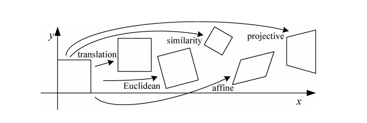
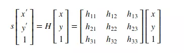
Suppose 1 pixel with coordinates (x, y) will be written as (x, y, 1). The coordinates (x, y, 1) are also equivalent to (xz, yz, z). The transformation of an image is equivalent to multiplying the coordinates of the points by a 3×3 H matrix of size. More details on Image Transformation can be found at: Image Alignment . Below is an illustration of transform by multiplying matrix H on a uniform coordinate system.
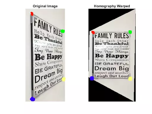
In image transformations, Perspective transform is a “magic” transformation, it does not preserve the angle, length, parallelism … but preserve the line. Also thanks to this property perspective transform helps us to transform an image from one perspective to another. Sounds a bit confusing, please look at the illustration below.
The photo on the left is a shot of a board taken off the left, the image on the right is the desired image obtained after transformation. First try to detect the coordinates of the four corners of the board, called source_points, and call the desired coordinates of the four corners in the output image as target_points. From two sets source_points and target_points, we can completely compute transform matrix H ( hormone matrix ). In this case, H is a Perspective transform matrix. Transforming the image with H, we get the image on the right, it looks like it was taken from a straight angle, it’s magical, right?
1.4.2 Estimate homography matrix with RANSAC.
Thus, if there are 4 points in the input image and 4 corresponding points in the target image, we can calculate the value of each element in matrix H. However, with the keypoint matching in section 1.3, we will obtain a constant. hundred pairs of points respectively [ ( k first , k first ′ ) , ( k 2 , k 2 ′ ) . . . ( k n , k n ′ ) ] [(k_1, k’_1), (k_2, k’_2) … (k_n, k’_n)] [(K 1 K 1 ‘ ), (K 2 , K 2 ‘ ) . . . (K n , K n ‘ ) ] . So choose which 4 pairs out of hundreds of other pairs of points to calculate H. Then we use the RANSAC algorithm.
RANSAC – Random Sample Consesus, is a fairly simple algorithm. In this problem, RANSAC simply samples any 4 pairs of random points, computes matrix H. Calculate the total difference between the target points and the input points after transforming by H. We have the formula
L o S S = Σ 0 n ( d i S S t a n c e ( H ∗ k i , k i ′ ) ) Loss = Sigma ^ n_0 (disstance (H * k_i, k’_i)) L o s s = Σ 0 n (D i s s t a n c e (H * k i , K i ‘ ) )
Inside, k i k_i k i and k i ′ k’_i k i ‘ is 1 pair of points respectively. Repeat sampling process – compute this loss with a sufficient number of times. Then choose H with the smallest Loss. Thus, we have obtained Homography matrix H used to convert the coordinates of the points in the input image to the target image. Opencv has provided a function to estimate matrix H
1 2 | H <span class="token operator">=</span> cv2 <span class="token punctuation">.</span> findHomography <span class="token punctuation">(</span> src_points <span class="token punctuation">,</span> dst_points <span class="token punctuation">,</span> cv2 <span class="token punctuation">.</span> RANSAC <span class="token punctuation">)</span> |
Thus we have obtained matrix H, used to convert the coordinates of the points in the input image to the coordinates of the corresponding points in the target image with the smallest error. Meanwhile, the input image has been transformed / merged into the target image to create a panorama image. Opencv has a convenient function for this image transformation:
1 2 | target_img <span class="token operator">=</span> cv2 <span class="token punctuation">.</span> warpPerspective <span class="token punctuation">(</span> src_img <span class="token punctuation">,</span> H_matrix <span class="token punctuation">,</span> <span class="token punctuation">(</span> w <span class="token punctuation">,</span> h <span class="token punctuation">)</span> <span class="token punctuation">)</span> |
2. Coding
The theory is a bit too much, now comes the visualization code. I will code as simple as possible. For convenience, I code on Google Colab, everyone can run / download the code from the following link: Google colab notebook: Image stitching.ipynb
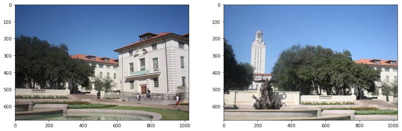
1 2 3 4 5 6 7 8 9 10 11 12 13 14 15 16 17 18 19 20 21 22 23 24 25 26 27 28 29 30 31 32 33 | <span class="token comment"># do các bản opencv mới nhất không có SIFT (có bản quyền) nên ta cần downgrad openCV</span> !pip uninstall opencv <span class="token operator">-</span> python <span class="token operator">-</span> y !pip install opencv <span class="token operator">-</span> contrib <span class="token operator">-</span> python <span class="token operator">==</span> <span class="token number">3.4</span> <span class="token number">.2</span> <span class="token number">.17</span> <span class="token operator">-</span> <span class="token operator">-</span> force <span class="token operator">-</span> reinstall <span class="token keyword">import</span> cv2 <span class="token keyword">import</span> numpy <span class="token keyword">as</span> np <span class="token keyword">import</span> matplotlib <span class="token punctuation">.</span> pyplot <span class="token keyword">as</span> plt <span class="token keyword">import</span> imutils <span class="token keyword">import</span> imageio <span class="token keyword">def</span> <span class="token function">plot_img</span> <span class="token punctuation">(</span> img <span class="token punctuation">,</span> size <span class="token operator">=</span> <span class="token punctuation">(</span> <span class="token number">7</span> <span class="token punctuation">,</span> <span class="token number">7</span> <span class="token punctuation">)</span> <span class="token punctuation">,</span> title <span class="token operator">=</span> <span class="token string">""</span> <span class="token punctuation">)</span> <span class="token punctuation">:</span> cmap <span class="token operator">=</span> <span class="token string">"gray"</span> <span class="token keyword">if</span> <span class="token builtin">len</span> <span class="token punctuation">(</span> img <span class="token punctuation">.</span> shape <span class="token punctuation">)</span> <span class="token operator">==</span> <span class="token number">2</span> <span class="token keyword">else</span> <span class="token boolean">None</span> plt <span class="token punctuation">.</span> figure <span class="token punctuation">(</span> figsize <span class="token operator">=</span> size <span class="token punctuation">)</span> plt <span class="token punctuation">.</span> imshow <span class="token punctuation">(</span> img <span class="token punctuation">,</span> cmap <span class="token operator">=</span> cmap <span class="token punctuation">)</span> plt <span class="token punctuation">.</span> suptitle <span class="token punctuation">(</span> title <span class="token punctuation">)</span> plt <span class="token punctuation">.</span> show <span class="token punctuation">(</span> <span class="token punctuation">)</span> <span class="token keyword">def</span> <span class="token function">plot_imgs</span> <span class="token punctuation">(</span> imgs <span class="token punctuation">,</span> cols <span class="token operator">=</span> <span class="token number">5</span> <span class="token punctuation">,</span> size <span class="token operator">=</span> <span class="token number">7</span> <span class="token punctuation">,</span> title <span class="token operator">=</span> <span class="token string">""</span> <span class="token punctuation">)</span> <span class="token punctuation">:</span> rows <span class="token operator">=</span> <span class="token builtin">len</span> <span class="token punctuation">(</span> imgs <span class="token punctuation">)</span> <span class="token operator">//</span> cols <span class="token operator">+</span> <span class="token number">1</span> fig <span class="token operator">=</span> plt <span class="token punctuation">.</span> figure <span class="token punctuation">(</span> figsize <span class="token operator">=</span> <span class="token punctuation">(</span> cols <span class="token operator">*</span> size <span class="token punctuation">,</span> rows <span class="token operator">*</span> size <span class="token punctuation">)</span> <span class="token punctuation">)</span> <span class="token keyword">for</span> i <span class="token punctuation">,</span> img <span class="token keyword">in</span> <span class="token builtin">enumerate</span> <span class="token punctuation">(</span> imgs <span class="token punctuation">)</span> <span class="token punctuation">:</span> cmap <span class="token operator">=</span> <span class="token string">"gray"</span> <span class="token keyword">if</span> <span class="token builtin">len</span> <span class="token punctuation">(</span> img <span class="token punctuation">.</span> shape <span class="token punctuation">)</span> <span class="token operator">==</span> <span class="token number">2</span> <span class="token keyword">else</span> <span class="token boolean">None</span> fig <span class="token punctuation">.</span> add_subplot <span class="token punctuation">(</span> rows <span class="token punctuation">,</span> cols <span class="token punctuation">,</span> i <span class="token operator">+</span> <span class="token number">1</span> <span class="token punctuation">)</span> plt <span class="token punctuation">.</span> imshow <span class="token punctuation">(</span> img <span class="token punctuation">,</span> cmap <span class="token operator">=</span> cmap <span class="token punctuation">)</span> plt <span class="token punctuation">.</span> suptitle <span class="token punctuation">(</span> title <span class="token punctuation">)</span> plt <span class="token punctuation">.</span> show <span class="token punctuation">(</span> <span class="token punctuation">)</span> src_img <span class="token operator">=</span> imageio <span class="token punctuation">.</span> imread <span class="token punctuation">(</span> <span class="token string">'http://www.ic.unicamp.br/~helio/imagens_registro/foto1A.jpg'</span> <span class="token punctuation">)</span> tar_img <span class="token operator">=</span> imageio <span class="token punctuation">.</span> imread <span class="token punctuation">(</span> <span class="token string">'http://www.ic.unicamp.br/~helio/imagens_registro/foto1B.jpg'</span> <span class="token punctuation">)</span> src_gray <span class="token operator">=</span> cv2 <span class="token punctuation">.</span> cvtColor <span class="token punctuation">(</span> src_img <span class="token punctuation">,</span> cv2 <span class="token punctuation">.</span> COLOR_RGB2GRAY <span class="token punctuation">)</span> tar_gray <span class="token operator">=</span> cv2 <span class="token punctuation">.</span> cvtColor <span class="token punctuation">(</span> tar_img <span class="token punctuation">,</span> cv2 <span class="token punctuation">.</span> COLOR_RGB2GRAY <span class="token punctuation">)</span> plot_imgs <span class="token punctuation">(</span> <span class="token punctuation">[</span> src_img <span class="token punctuation">,</span> tar_img <span class="token punctuation">]</span> <span class="token punctuation">,</span> size <span class="token operator">=</span> <span class="token number">8</span> <span class="token punctuation">)</span> |
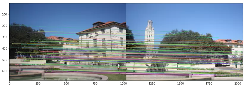
1 2 3 4 5 6 7 8 9 10 11 12 13 14 15 16 17 18 19 20 21 22 23 24 25 26 | SIFT_detector <span class="token operator">=</span> cv2 <span class="token punctuation">.</span> xfeatures2d <span class="token punctuation">.</span> SIFT_create <span class="token punctuation">(</span> <span class="token punctuation">)</span> kp1 <span class="token punctuation">,</span> des1 <span class="token operator">=</span> SIFT_detector <span class="token punctuation">.</span> detectAndCompute <span class="token punctuation">(</span> src_gray <span class="token punctuation">,</span> <span class="token boolean">None</span> <span class="token punctuation">)</span> kp2 <span class="token punctuation">,</span> des2 <span class="token operator">=</span> SIFT_detector <span class="token punctuation">.</span> detectAndCompute <span class="token punctuation">(</span> tar_gray <span class="token punctuation">,</span> <span class="token boolean">None</span> <span class="token punctuation">)</span> <span class="token comment">## Match keypoint</span> bf <span class="token operator">=</span> cv2 <span class="token punctuation">.</span> BFMatcher <span class="token punctuation">(</span> cv2 <span class="token punctuation">.</span> NORM_L2 <span class="token punctuation">,</span> crossCheck <span class="token operator">=</span> <span class="token boolean">False</span> <span class="token punctuation">)</span> <span class="token comment">## Bruce Force KNN trả về list k ứng viên cho mỗi keypoint. </span> rawMatches <span class="token operator">=</span> bf <span class="token punctuation">.</span> knnMatch <span class="token punctuation">(</span> des1 <span class="token punctuation">,</span> des2 <span class="token punctuation">,</span> <span class="token number">2</span> <span class="token punctuation">)</span> matches <span class="token operator">=</span> <span class="token punctuation">[</span> <span class="token punctuation">]</span> ratio <span class="token operator">=</span> <span class="token number">0.75</span> <span class="token keyword">for</span> m <span class="token punctuation">,</span> n <span class="token keyword">in</span> rawMatches <span class="token punctuation">:</span> <span class="token comment"># giữ lại các cặp keypoint sao cho với kp1, khoảng cách giữa kp1 với ứng viên 1 nhỏ hơn nhiều so với khoảng cách giữa kp1 và ứng viên 2</span> <span class="token keyword">if</span> m <span class="token punctuation">.</span> distance <span class="token operator"><</span> n <span class="token punctuation">.</span> distance <span class="token operator">*</span> <span class="token number">0.75</span> <span class="token punctuation">:</span> matches <span class="token punctuation">.</span> append <span class="token punctuation">(</span> m <span class="token punctuation">)</span> <span class="token comment"># do có cả nghìn match keypoint, ta chỉ lấy tầm 100 -> 200 cặp tốt nhất để tốc độ xử lí nhanh hơn</span> matches <span class="token operator">=</span> <span class="token builtin">sorted</span> <span class="token punctuation">(</span> matches <span class="token punctuation">,</span> key <span class="token operator">=</span> <span class="token keyword">lambda</span> x <span class="token punctuation">:</span> x <span class="token punctuation">.</span> distance <span class="token punctuation">,</span> reverse <span class="token operator">=</span> <span class="token boolean">True</span> <span class="token punctuation">)</span> matches <span class="token operator">=</span> matches <span class="token punctuation">[</span> <span class="token punctuation">:</span> <span class="token number">200</span> <span class="token punctuation">]</span> img3 <span class="token operator">=</span> cv2 <span class="token punctuation">.</span> drawMatches <span class="token punctuation">(</span> src_img <span class="token punctuation">,</span> kp1 <span class="token punctuation">,</span> tar_img <span class="token punctuation">,</span> kp2 <span class="token punctuation">,</span> matches <span class="token punctuation">,</span> <span class="token boolean">None</span> <span class="token punctuation">,</span> flags <span class="token operator">=</span> cv2 <span class="token punctuation">.</span> DrawMatchesFlags_NOT_DRAW_SINGLE_POINTS <span class="token punctuation">)</span> plot_img <span class="token punctuation">(</span> img3 <span class="token punctuation">,</span> size <span class="token operator">=</span> <span class="token punctuation">(</span> <span class="token number">15</span> <span class="token punctuation">,</span> <span class="token number">10</span> <span class="token punctuation">)</span> <span class="token punctuation">)</span> <span class="token comment">## Nhìn vào hình dưới đây, ta thấy các cặp Keypoint giữa 2 ảnh đã được match khá chính xác, số điểm nhiễu không quá nhiều</span> |
Estimate Homography matrix and Transform Image
1 2 3 4 5 6 7 8 9 10 11 12 13 | kp1 = np.float32([kp.pt for kp in kp1]) kp2 = np.float32([kp.pt for kp in kp2]) pts1 = np.float32([kp1[m.queryIdx] for m in matches]) pts2 = np.float32([kp2[m.trainIdx] for m in matches]) # estimate the homography between the sets of points (H, status) = cv2.findHomography(pts1, pts2, cv2.RANSAC) print(H) => [[ 7.74666572e-01 2.97937348e-02 4.48576839e+02] [-1.31635664e-01 9.10804272e-01 7.63230050e+01] [-2.03305884e-04 -3.33235166e-05 1.00000000e+00]] |
Transform image
1 2 3 4 5 6 | h1 <span class="token punctuation">,</span> w1 <span class="token operator">=</span> src_img <span class="token punctuation">.</span> shape <span class="token punctuation">[</span> <span class="token punctuation">:</span> <span class="token number">2</span> <span class="token punctuation">]</span> h2 <span class="token punctuation">,</span> w2 <span class="token operator">=</span> tar_img <span class="token punctuation">.</span> shape <span class="token punctuation">[</span> <span class="token punctuation">:</span> <span class="token number">2</span> <span class="token punctuation">]</span> result <span class="token operator">=</span> cv2 <span class="token punctuation">.</span> warpPerspective <span class="token punctuation">(</span> src_img <span class="token punctuation">,</span> H <span class="token punctuation">,</span> <span class="token punctuation">(</span> w1 <span class="token operator">+</span> w2 <span class="token punctuation">,</span> h1 <span class="token punctuation">)</span> <span class="token punctuation">)</span> result <span class="token punctuation">[</span> <span class="token number">0</span> <span class="token punctuation">:</span> h2 <span class="token punctuation">,</span> <span class="token number">0</span> <span class="token punctuation">:</span> w2 <span class="token punctuation">]</span> <span class="token operator">=</span> tar_img plot_img <span class="token punctuation">(</span> result <span class="token punctuation">,</span> size <span class="token operator">=</span> <span class="token punctuation">(</span> <span class="token number">20</span> <span class="token punctuation">,</span> <span class="token number">10</span> <span class="token punctuation">)</span> <span class="token punctuation">)</span> |
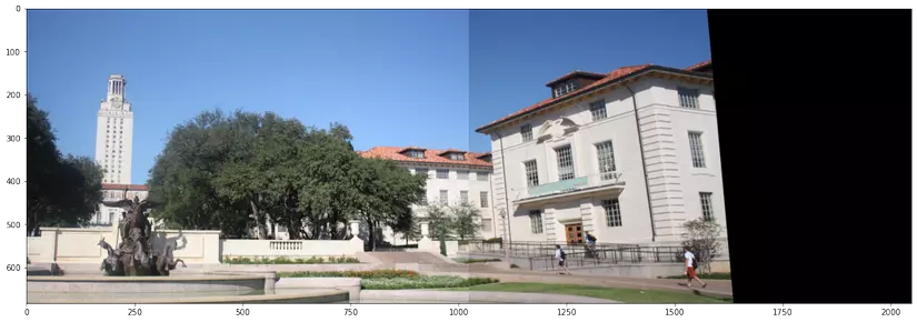
Thus, with just a few lines of code we can stitch 2 images together. The resulting photo also looks quite reasonable, right. Actually, if you pay close attention, the colors between the two parts that are merged look a little different. In practice, one has to use post-processing methods to remedy this situation. However, due to the length of the article, I would like to stop here. Thank you for reading this article