Title

Did you know that, to teach machine learning a model, we emit up to five times more carbon than a car over the course of its life cycle ? So let’s see what we can do with that model for what environmental destruction.

As you probably know, the starting point of the weights in a model has a significant effect on machine learning results. If you start in a remote place, it will be difficult and it takes a long time to reach the promised land. If you start with a temporary matrix (using Xavier / Glorot initialization ) then the model will not be returned.

0 0$0$ (vanishing gradient) or

∞ infty$\infty$

According to the policy of 3R (Reduce-Reuse-Recycle), as the above idea, we will reuse the model already trained to do other things. Not only saves resources for environmental protection, better quality than new train from the beginning, has just been a Viblo article to write.

Note : we need to do both things, not leave job 1 through work 2. In the fly fan example above, we want to fan the instruments and chase the flies. The summer is very hot.

If you can copy the fan

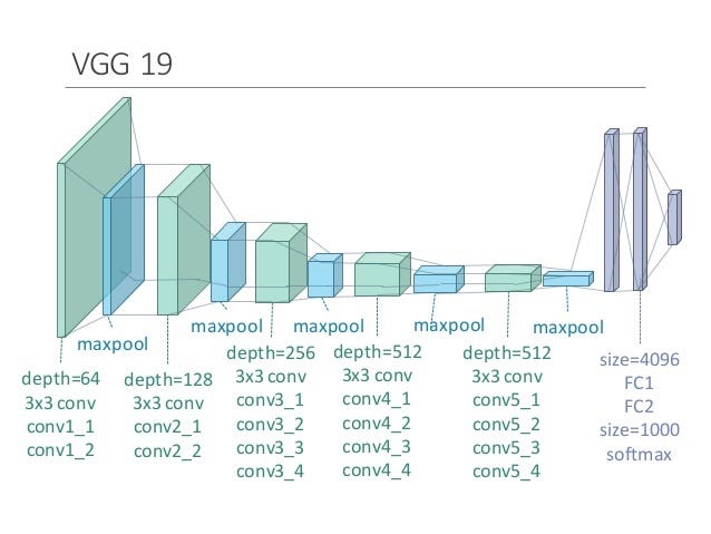
The title is meme derived from here . If you do not understand / do not know, then ignore me, I’m very pale. And the artwork is standard VGG only.

Just like 3D printing a new fan, you Ctrl + C Ctrl + V your existing model to go to work. Assuming you use a face recognition model to identify sausages, for example, what do you need to do? Quite sure you’ve heard the term transfer learning – if not then don’t worry, that’s the subject of this section! We will list out the basic methods you can use:

Feature Extraction

That is when you use the network (eg CNN / VGG) just to separate the depth characteristics only. From the learned web, you keep (freezing) the entire weight until the class right before softmax – the 1000-dimensional vector that will be the extracted features. Then you just replace the final softmax layer to predict the sausage instead of the face.

Fine-tuning

You did not freeze anything. Using the trained model to identify faces as the starting point, teach it to identify whether it is a sausage. Maybe you choose a low learning rate so it doesn’t go too far away from what it already knows. Or you can freeze the first few layers and just tweak the last few layers; it’s a bit similar to the aforementioned feature extraction.

And if you have to reuse the fan

… then at least you can fold it to smash somebody.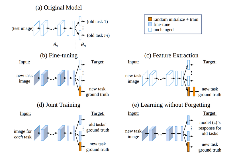

Revise the basic method above

We still use the network by specific extraction or refining method, but instead of copying the whole network into 2, we just add another softmax class for its new task. However, you probably also realize that by using old weights / teaching weights over it, the quality of the models will go down. So what to do?

Teaching both (Joint Training / Multitask Learning)

After you have created two heads for the model, you occasionally apply a spoon of face image data, occasionally inserting a spoon of sausage data (and changing the corresponding output being taught). If you do that, the model will be learned evenly so that it does both of the work in the most balanced way. However, the problem is that there is not always data of the original model, so how now?

Learning not to forget! (Learning without Forgetting)

Without the original model data, we just need to create that data. Taking the inputs for the new model and calculating the results with the old model will give you a new output that replaces ground truth – vila, you’ve got a data set that replaces the original data set. Also, by reusing the data set of the new task instead of re-training on the data of the old task, you don’t have to train your model on more data than in the “teach both.”

Attention! Math forward. Can skip paragraphs, just formulas. The difference can be seen when the quality balance of the two models of the LwF method falls within the same loss function (temporarily reduced the weight decay for simplicity):

L = λ 0 L o l d ( Y o , Y ^ o ) + L n e w ( Y n , Y ^ n ) , mathcal {L} = lambda_0 mathcal {L} _ {old} (Y_o, hat {Y} _o) + mathcal {L} _ {new} (Y_n, hat {Y} _n),

$$\mathcal{L}={\lambda }^0{\mathcal{L}}^{old}{(Y}^o{\hat{Y}}^o)+{\mathcal{L}}^{new}{(Y}^n{\hat{Y}}^n),$$

with the first part being the loss function for the old model (

Y ^ o hat {Y} _o

${\hat{Y}}^o$ is the output of the old model for the new input), the latter is the loss function for the new model, and parameters

$\lambda$ $0$ $lambda\_0$

λ 0 control whether you want to focus on keeping the quality of older models or focus on teaching newer models.

Comparison between the above methods:

Spring Weight (Elastic Weight Consolidation)

The basic idea of ​​EWC is similar to LwF, however more important weights will be retained. This part is a lot of math, so you can skip it if the general explanation above is enough for you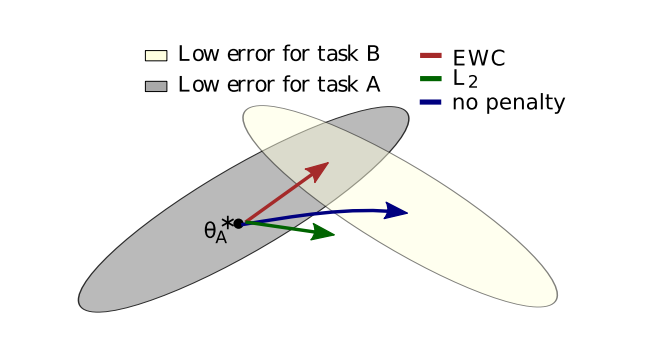

The article, easy to explain, is a generic linear network used for classification (giving probability 0/1). Since train a model is to find the most appropriate weights (highest probabilities) for the data we have, we need to maximize the probability.

p ( θ ∣ D ) p ( theta vert D)

$p(\theta |D)$ , or its equivalent (because the log function is an incremental function). Using Bayes’ rule, we have

log ⁡ p ( θ ∣ D ) = log ⁡ p ( D ∣ θ ) + log ⁡ p ( θ ) – log ⁡ p ( D ) . ( first ) log p ( theta vert mathcal {D}) = log p (D vert theta) + log p ( theta) – log p (D). (first)

lo g p ( θ ∣ D ) = lo g p ( D ∣ θ ) + lo g p ( θ ) – lo g p ( D ) . ( 1 )

Divide data into 2 parts

D A SKIN

$D^A$ and

$D$ $B$ $D\_B$

D B , where A is the first task we learned weights, and B is the new task we have

log ⁡ p ( θ ∣ D ) = log ⁡ p ( D A ∣ θ ) + log ⁡ p ( D B ∣ θ ) + log ⁡ p ( θ ) – log ⁡ p ( D A ) – log ⁡ p ( D B ) , ( 2 ) log p ( theta vert mathcal {D}) = log p (D_A vert theta) + log p (D_B vert theta) + log p ( theta) – log p (D_A ) – log p (D_B), (2)

lo g p ( θ ∣ D ) = lo g p (D A ∣ θ ) + lo g p (D B ∣ θ ) + lo g p ( θ ) – lo g p (D A ) – lo g p (D B ) , ( 2 )

and then replace

D D

$D$ in equation (1) with

D A SKIN

$D^A$

log ⁡ p ( θ ∣ D ) = log ⁡ p ( θ ∣ D A ) + log ⁡ p ( D B ∣ θ ) – log ⁡ p ( D B ) . log p ( theta vert mathcal {D}) = log p ( theta vert D_A) + log p (D_B vert theta) – log p (D_B).

lo g p ( θ ∣ D ) = lo g p (θ | D A ) + lo g p (D B ∣ θ ) – lo g p (D B ) .

Notice that

log ⁡ p ( D ∣ θ ) = – L ( D , θ ) log p (D vert theta) = – L (D, theta)

lo g p ( D ∣ θ ) = – L ( D , θ ) , with

$L$ $L$

L is the loss function of the classification problem (negative log-likelihood, you can learn more here , and here ). From the above formula, you can see that, to optimize a dual network, we only need to minimize the loss function of the new task plus some weight importance representations according to the original data task (and

$log$ $$ $p$ $($ $D$ $B$ $)$ $log\; p\; (D\_B)$

lo g p (D B ) is unrelated to the problem and can be considered a constant). We estimate

$log$ $$ $p$ $($ $\theta$ $|$ $D$ $A$ $)$ $log\; p\; (\; theta\; vert\; D\_A)$

lo g p (θ | D A ) using Laplace transformation with Fisher information matrix

$F$ $F$

F :

log ⁡ p ( θ ∣ D A ) ≈ ∑ i F i 2 ( θ i – θ i , A ∗ ) 2 . log p ( theta vert D_A) approx sum_i frac {F_i} {2} left ( theta_i- theta_ {i, A} ^ * right) ^ 2.

lo g p (θ | D A ) ≈ i Σ 2 F i (Θ i – θ i, A * ) 2 .

Matrix

F F

$f$ will determine the weighting

i i

$i$

log ⁡ p ( θ ) log p ( theta)

lo g p ( θ ) is a constant), put it all together, we have

L ( θ ) = L B ( θ ) + λ ∑ i F i 2 ( θ i – θ i , A ∗ ) 2 , mathcal {L} ( theta) = L_B ( theta) + lambda sum_i frac {F_i} {2} left ( theta_i- theta_ {i, A} ^ * right) ^ 2,

$$\mathcal{L}(\theta )=L^B(\theta )+\lambda \stackrel{\Sigma }{i}\genfrac{}{}{0ex}{}{F^i}{2}$$ (Θ i – θ i, A * ) 2 ,

with

λ lambda

$\lambda$ control the weight rate away from the optimization of the original task.

If you are big again

If you survived the math, I would like to ask for one because I still do not fully understand the Laplace transform for the probability domain and Fisher information matrix. I bring the good news to you: the math has come to an end, and from here on all the deep learning (and we know that there is not much math in deep learning …)

The following methods will use the fact that models usually have a majority of weights close to zero, and use pruning methods to make room in the model to accommodate another similar model. Regarding pruning, you can refer to the shortened version here , a pretty good article by Pham Huu Quang (just read Pruning!); or the long version here , an article from his boss Pham Van Toan.

PackNet

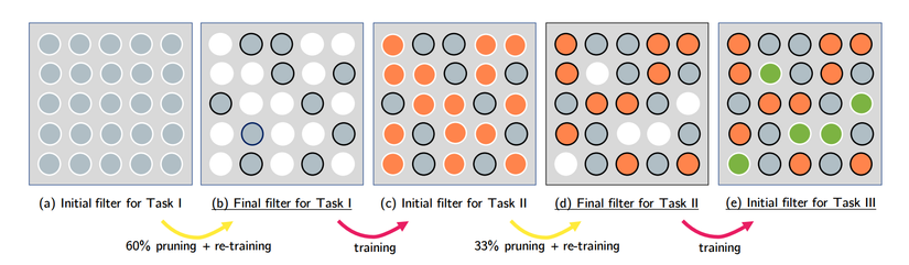
As illustrated above, from a model with lots of parameters we train for task 1, we prune (set to 0) some parameters. After that, we just train the parameter to zero (and freeze where the weight is kept unchanged) for task 2 (note that task 2 is still using the weight learned from task 1). ). After that, we again prune part weight of task 2, jump over task 3, and so on until all weights are closed.

Choosing weights to retain can be understood as a parameterized estimation of EWC, when instead of changing weights according to their importance, we always choose a fixed number of weights. key numbers to stay the same, and the others to be taught from scratch. At the same time, the actual test results show that removing 95% of the model’s weight even increases their quality (!); and reusing cells retained for the next task can be considered as a version of transfer learning, when the most important information learned is passed on to the next generation.

Regarding personal thoughts, there are some points they did not mention in the article that interest me.

(?) Why do they prune that weight instead of just masking them when they train, leaving behind the little knowledge they have learned?
(!) They probably keep the model from getting stuck at a local minimum.

(?) Why are they not just for tasks

n n

$n$ using some (instead of all) weights learned from previous tasks?
(!) Maybe it’s because it’s so hard ¯ _ (ツ) _ / ¯

Piggyback

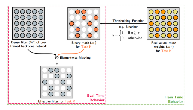
2 of the 3 authors of this article are 2/2 the authors of the original PackNet article, so you will probably guess right away that this is a better improvement model of the aforementioned model. However, no … This model trains a layer of 0/1 mask over a root network (VGG-16 / ResNet-50) for each task to be done, using a weight of 0/1 selection threshold – It is easy to realize that this mask class is derivative. The idea is simple, but the article is long and unnecessary, so please read through it. Not to mention, if only filtering out the weights to create a new network (without retrain the selected weights) and achieving better results than optimizing the full network is a bit hard to believe (or maybe it’s true and I just lack of faith). Anyway, I still listed this website for this comprehensive article.

Results and reference sources

At this point, I’m out of martial arts. If you have any more, please leave me below the comment. At the same time, I am stuck with ideas for articles / research / dissertations, so if you ask the noble people, please do not share, I promise you will have the full credit = ((Thank you and make an appointment you next month!

And the following is the article the author had to cry while reading to write this article:

Learning without Forgetting:
https://arxiv.org/pdf/1606.09282.pdf

Elastic Weight Consolidation:
https://arxiv.org/pdf/1612.00796.pdf

PackNet:
https://arxiv.org/pdf/1711.05769.pdf

Piggyback:
https://arxiv.org/pdf/1801.06519.pdf