History of Deep Learning

Introduce

Artificial intelligence is making its way into our lives and deeply influences us. Ever since I wrote the first article, the frequency with which we hear the words ‘artificial intelligence’, ‘machine learning’ and ‘deep learning’ has been increasing. The main reason for this (and the creation of this blog) is the appearance of deep learning in the last 5-6 years.

Once again, please use the drawings depicting the relationship between artificial intelligence, machine learning, and deep learning:

The relationship between AI, Machine Learning and Deep Learning.
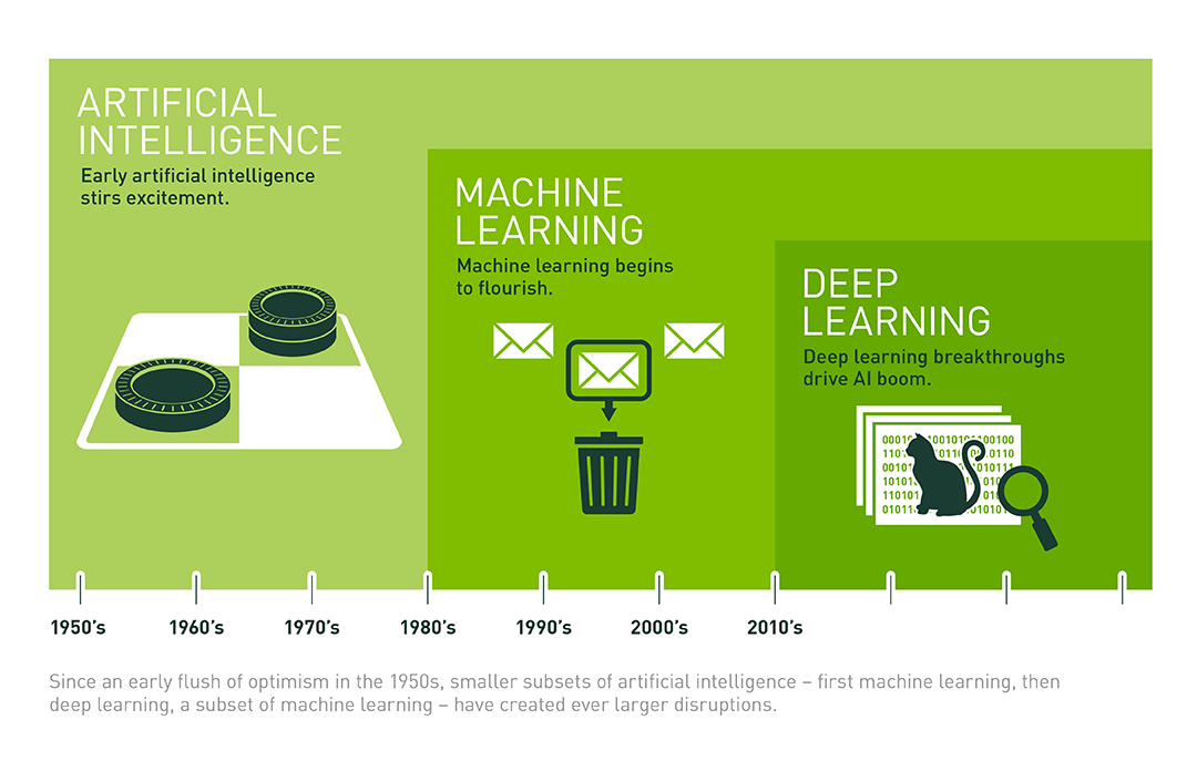
(Source: What’s the Difference Between Artificial Intelligence, Machine Learning, and Deep Learning? )

In this article, I will briefly outline the history of deep learning. In the following articles, I am ambitious to write carefully about the basic components of deep learning systems. Further, the blog will have tutorials for many practical problems.

The blog always receives contributions to improve the quality of the articles. If you have any contributions, please leave in the comment section, I will update the post accordingly. Thank you.

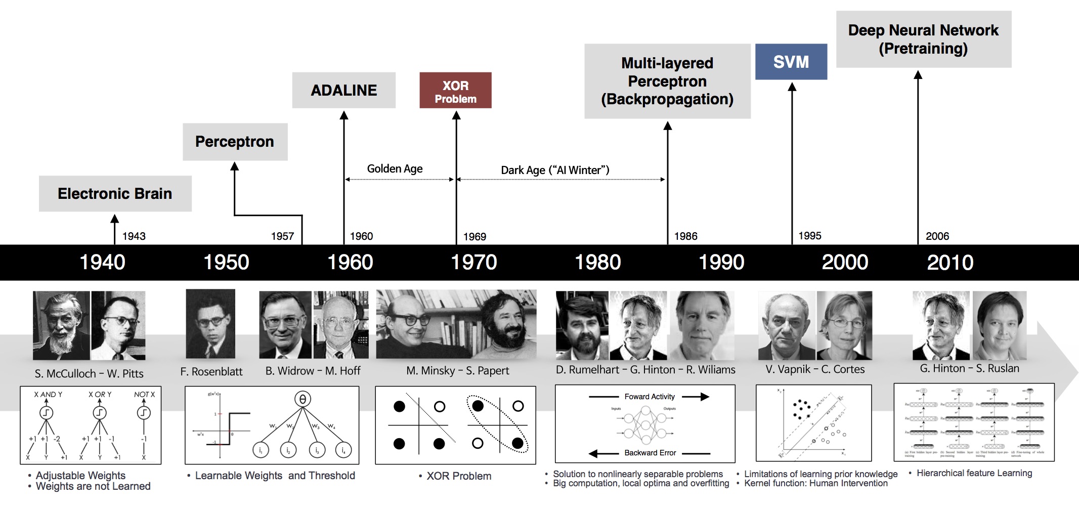
Important milestones of deep learning

Deep learning has been mentioned a lot in recent years, but the basic foundations have been around for a long time …

Let’s look at the image below:

Deep learning history (Source: Image is taken from Deep Learning 101 – Part 1: History and Background . The author of the article doesn’t know the exact origin of the image.)

Perceptron (60s)

One of the first foundations of neural networks and deep learning is the perceptron learning algorithm (or perceptron for short). Perceptron is a supervised learning algorithm that solves the binary classification problem, originated by Frank Rosenblatt in 1957 in a study funded by the U.S. Naval Research Office (US Office of Naval Research – from a military-related agencies ). The perceptron algorithm is proven to converge if the two data layers are linearly separable . With this success, in 1958, in a workshop, Rosenblatt made a controversial speech. From this statement, the New York Times reported an article that the perceptron was expected by the US Navy to “be able to walk, talk, look, write, reproduce, and be aware of its existence.” ”. ( We know that up to many times more perceptron systems have not been able to .)

Although this algorithm brought many expectations, it quickly proved impossible to solve simple problems. In 1969, Marvin Minsky and Seymour Papert in the famous book Perceptrons proved that it is impossible to ‘learn’ the XOR function when using perceptrons. This discovery stunned the scientific world at the time ( we now see this fairly obvious ). Perceptron is proven to work only if the data is linearly separable .

This finding caused the study of perceptrons to be interrupted for nearly 20 years. This period is also known as The First AI winter .

Until…

MLP and Backpropagation are born (80s)

Geoffrey Hinton graduated with a PhD in neural networks in 1978. In 1986, he and two other authors published a scientific paper in Nature entitled “Learning representations by back-propagating errors” . In this paper, his team demonstrated that neural nets with many hidden layers (called multi-layer perceptrons or MLPs) can be effectively trained based on a simple process called backpropagation ( backpropagation). This is the beautiful name of the chain rule – in the derivative, it is important to calculate the derivative of the complex function that describes the relationship between the input and output of a neural net. The optimal algorithm is all done through derivative calculation, gradient descent is an example .) This helps the neural nets escape perceptron’s limitations of only representing linear relationships. To represent nonlinear relationships, behind each layer is a nonlinear activation function, for example sigmoid or fishy functions. (ReLU was born in 2012). With hidden layers, neural nets have been shown to be capable of approximating almost any function through a theorem called a universal approximation theorem . Neurel nets return to the game .

This algorithm brought a few initial successes, notably the convolutional neural nets (convnets or CNN) (also known as LeNet ) for the handwriting recognition problem originated by Yann LeCun at AT&T Bell Labs ( Yann LeCun was a graduate student of Hinton at the University of Toronto in 1987-1988). Below is a demo taken from LeNet’s website, the network is a CNN with 5 layers, also known as LeNet-5 (1998).

LeNet-5 for handwriting recognition problem. (Source: http://yann.lecun.com )

This model is widely used in handwritten number reading systems on bank checks and postal codes of the United States.

LeNet was the best algorithm of the time for the problem of handwritten image recognition. It is better than regular MLP (with fully connected layer) because it has the ability to extract features in two dimensions of the image through two-dimensional filters. Moreover, these filters are small so the storage and calculation are also better than regular MLP. ( Yan LeCun comes from Electrical Engineering so is very familiar with filters. )

Second AI Winter (90s – early 2000s)

Similar models are expected to solve many other image classification problems. However, unlike the digits, other types of photos were very limited because digital cameras were not popular at the time. Reappears photos as rare. While in order to train convnets, we need a lot of training data. Even when the data was sufficient, another dilemma was that the computing power of the computers at that time was very limited.

Another limitation of MLP architectures in general is that the loss function is not a convex function. This makes it very difficult to find the optimal optimal solution for the optimal problem of loss function. Another problem related to the computing limits of computers also makes MLP training inefficient when the number of hidden layers increases. This problem is called vanishing gradient .

Recall that the trigger function used that time is sigmoid or fishy – are functions that are blocked between (0, 1) or (-1, 1) (Recall the sigmoid derivative $\sigma \left(z\right)$ is $\sigma \left(z\right)(1–\sigma (z\left)\right)$ is the product of two numbers less than 1). When using backpropagation to calculate the derivative for coefficient matrices in the first class, we need to multiply lots of values ​​less than 1 together. This causes many component derivatives to be zero due to the approximation. When the derivative of an element is zero, it will not be updated via gradient descent!

These limitations caused neural nets once again to become ice age . In the 1990s and early 2000s, neural nets were gradually replaced by support vector machines –SVM. SVMs have the advantage that the optimal problem to find its parameters is a convex problem – there are many effective optimization algorithms to help find its solution. The kernel techniques have also evolved to help SVMs solve both the problem of non-linear data.

Many machine learning scientists turned to SVM research during that time, except for a few stubborn scientists …

The name has been renewed – Deep Learning (2006)

In 2006, Hinton again said that he knew the brain activity how , and introduced the idea of money coaching unattended ( unsupervised pretraining ) through deep nets Belief (DBN) . DBN can be viewed as a superposition of unsupervised networks such as restricted Boltzman machines or autoencoders .

Take for example with autoencoder. Each autoencoder is a neural net with a hidden layer. The number of hidden units is less than the number of input units, and the number of output units is equal to the number of input units. This network is simply trained so that the output layer results are the same as the input layer results (and therefore called the autoencoder). The process of data going from the input layer to the hidden layer can be considered as coding , the process of data going from the hidden layer to the output layer can be considered decoding . When the output is similar to the input, we can see that the hidden layer with fewer units has been able to encode the input quite successfully, and can be considered to have the properties of the input. If we abandon the output layer, fixed (freeze) the connection between input and hidden layers, the hidden layer output as a new input, and then coaching a different autoencoder, we added a new layer hidden. This process continues for a long time to get a deep enough network that the output of this large network (which is the hidden layer of the last autoencoder) carries the information of the initial input. Then we can add other layers depending on the problem (eg add softmax layer at the end for classification problem). The whole network trained a few more epochs. This process is known as refining (fine tuining).

Why is this training process so beneficial?

One of the mentioned limitations of MLP is the vanishing gradient problem. Weighting matrices for the first layer of the network are difficult to train because the derivative of the loss function according to these matrices is small. With DBN’s idea, weighting matrices in the first hidden layers are pre-trained ( pretrained ). These pre-trained weights can be considered a good initial value for the top hidden layers. This helps somewhat avoid the hassle of vanishing gradients .

From here on, neural networks with many hidden layers have been renamed to deep learning .

The vanishing gradient problem is somewhat solved (not really thorough yet), but there are still other deep learning issues: training data is too little, and CPU computation is very limited in training. train deep networks.

In 2010, Professor Fei-Fei Li, a leading professor of computer vision at Stanford, together with her team created a database called ImageNet with millions of images belonging to 1,000 different data layers. stick the sticker. This project was implemented thanks to the boom of the internet in the 2000s and the huge amount of photos uploaded to the internet at that time. These photos are labeled by a lot of people (paid).

See also How we teach computers to understand pictures. Fei-Li Fei

This database is updated every year, and since 2010, it has been used in an annual contest called ImageNet Large Scale Visual Recognition Challenge (ILSVRC) . In this competition, training data is given to participating teams. Each team needs to use this data to train classification models, which will be applied to predict the label of new data (held by the organizers). In 2010 and 2011, many teams participated. These two-year models are mainly a combination of SVM with features built by hand-crafted descriptors (SIFT, HoG, etc.). The winning model has a top-5 error rate of 28% (the smaller the better). The model that won in 2011 had a top-5 error rate of 26%. Not much improvement!

Margins: top-5 error rate is calculated as follows. Each model predicts 5 labels of a photo. If the actual label of the image is in those 5, we have an accurate layered point. Also, that image is considered an error. Top-5 error rate is the ratio of the number of error images in the entire test image to the error calculated in this way. Top-1 error plus classification accuracy (percent) is equal to 100 percent.

Breakthrough (2012)

In 2012, also at ILSVRC, Alex Krizhevsky, Ilya Sutskever, and Geoffrey Hinton (again him) participated and achieved a top-5 error rate of 16%. This result stunned researchers about that time. The model is a Deep Convolutional Neural Network, later known as AlexNet .

In this paper, many new techniques are introduced. The two most prominent contributions are ReLU and dropout. The function ReLU ( $\text{ReLU}\left(x\right)=max(x,0)$ ) with simple calculations and derivatives (equal to 1 when the input is not negative, equal to 0 when vice versa) helps Training speed increased significantly. In addition, the fact that ReLU is not blocked by 1 (such as softmax or fishy) makes the vanishing gradient problem somewhat solved. Dropout is also a simple and extremely effective technique. During the training, many hidden units are randomly turned off and the model is trained on the remaining parameter sets. During the test, all units will be used. This approach is quite reasonable when compared to humans. If using only a part of the energy that has brought about an effect, using the whole energy will be more effective. This also helps the model avoid overfitting and is similar to the ensemble technique in other machine learning systems. For each way off units, we have a different model. With many different combinations of units off, we get a lot of models. The combination at the end is considered to be a combination of multiple models (and thus, it is similar to ensemble learning ).

One of the most important factors that helps AlexNet succeed is the use of GPU (graphics card) to train the model. The GPU created for gamers, with the ability to run multiple cores in parallel, has become an extremely suitable tool for deep learning algorithms, helping to accelerate the algorithm many times over the CPU.

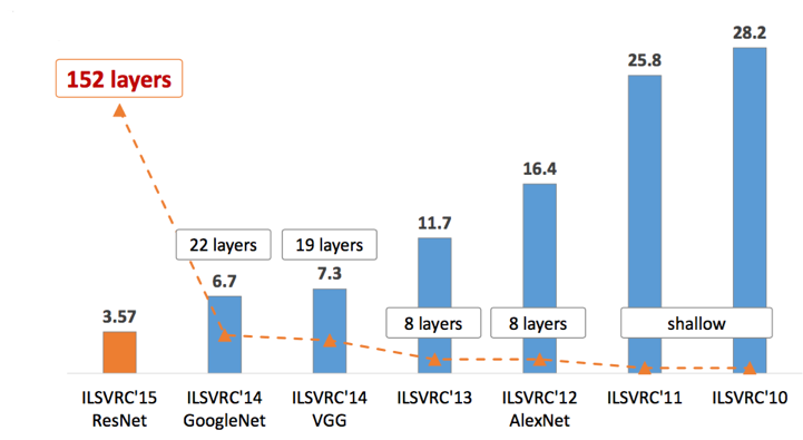
After AlexNet, all models that won high prizes in the following years are deep networks (ZFNet 2013, GoogLeNet 2014, VGG 2014, ResNet 2015). I will take a blog post to write about these important architectures. General trend can be seen as models of increasingly deep. See image below.

ILSVRC results over the years. (Source: CNN Architectures: LeNet, AlexNet, VGG, GoogLeNet, ResNet and more … )

Big tech companies are also interested in developing deep learning labs during this time. Many groundbreaking technology applications have been applied to everyday life. Also since 2012, the number of scientific articles on deep learning has increased exponentially. Deep learning blogs are also increasing day by day.

What brings the success of deep learning?

Many of the basic ideas of deep learning were laid down in the 80-90s of the last century, but deep learning has only been breaking through for 5-6 years. Why?

There are many factors that led to this boom:

• The introduction of labeled big data sets
• High-speed parallel computing capability of GPU.
• The introduction of ReLU and the related activation functions limited the vanishing gradient problem.
• Improvements of architectures: GoogLeNet, VGG, ResNet, … and transfer learning techniques, fine tuning.
• Many new regularization techniques: dropout, batch normalization, data augmentation.
• Many new libraries support deep network training with GPUs: theano, caffe, mxnet, tensorflow, pytorch, keras, …
• Many new optimization techniques: Adagrad, RMSProp, Adam, …

Conclude

Many readers have asked me to write about deep learning for a long time. However, before that, I realized that I did not have enough knowledge in this field to write for readers. Only when I had a basic understanding of machine learning and I had accumulated a certain amount of knowledge did I decide to start on this topic of interest.

Other classic machine learning algorithms can still appear in future articles of the blog.

Source : Techtalk