MFCC – Mel frequency cepstral coefficients
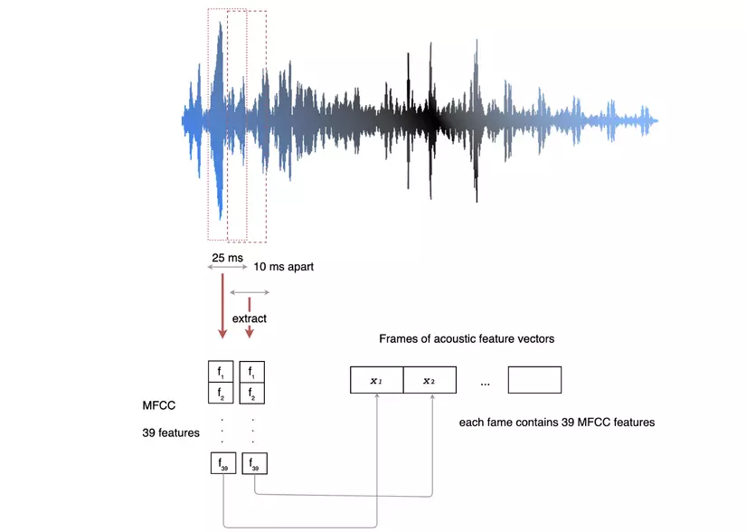
In this article, I will focus on converting voice signals into MFCC format – commonly used in Speech recognition and many other related speech problems. We can imagine the MFCC calculation by processing flow: cutting the audio signal sequence into equal short segments (25ms) and overlap (10ms). Each of these audio segments is modified, calculated to gain 39 features. Each list of 39 features has high independence, low noise, small enough to ensure computation, enough information to ensure the quality of identification algorithms.
The following figure shows the flow of processing from the audio input ⟶ longrightarrow ⟶ MFCC
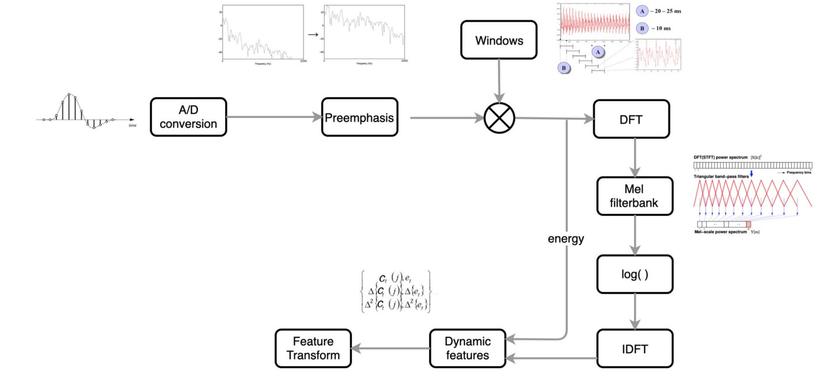
1. A / D Conversion and Pre-emphasis
1.1 A / D Conversion
Sound is a continuous signal, while computers work with discrete numbers. We need to take samples at evenly spaced intervals with a specified sampling rate (sample rate) to convert from a continuous signal form to a discrete form. For example sample_rate = 8000 ⟶ longrightarrow ⟶ in 1s takes 8000 values.
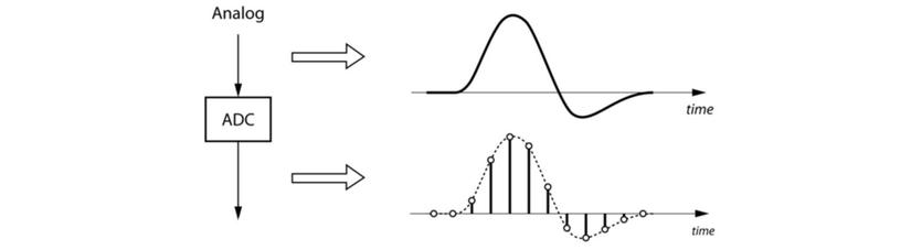
The human ear hears sounds in the 20Hz range → big → 20,000 Hz. According to the Nyquist – Shannon sampling theorem : with a signal with component frequencies ≤ f m leq f_m ≤ f m , to ensure that sampling does not cause loss of information (aliasing), sampling frequency f S f_s f s Make sure f S ≥ 2 f m f_s geq 2f_m f s ≥ 2 f m .
So to ensure that sampling does not cause loss of information, sampling frequency f S = 44100 H z f_s = 44100 Hz f s = 4 4 1 0 0 H z . However in many cases, people just need to take f S = 8000 H z f_s = 8000Hz f s = 8 0 0 0 H z or f S = 16000 H z f_s = 16000Hz f s = 1 6 0 0 0 H z .
1.2. Pre-emphasis
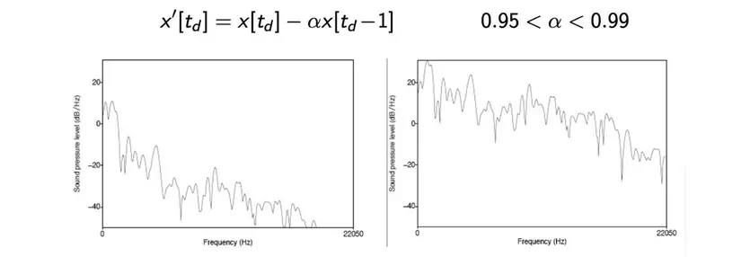
Due to the characteristics of larynx and vocalization, our voices are characterized: low-frequency sounds with high energy levels, high-frequency sounds with relatively low energy levels. Meanwhile, these high frequencies still contain a lot of phonological information. So we need a pre-emphasis step to trigger these high frequency signals.
2. Spectrogram
2.1 Windowing
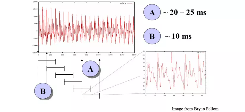
Instead of transforming Fourier on a long audio track, we slide a window along the signal to retrieve the frames and then apply DFT on each of these frames (DFT – Discrete Fourier Transform). Because the average human speech speed is about 3, 4 words per second, the width of each frame is about 20 – 25ms. The frames are overlap around 10ms to capture the changing context.
However, cutting the frame will cause the values at the two edges of the frame to drop dramatically (to zero), which will lead to the phenomenon: when DFT enters the frequency domain there will be a lot of noise at high frequencies. To fix this, we need to smooth it by multiplying the frame by several window types. There are several common types of window, such as Hamming window, Hanning window, etc. that work to reduce the frame border value slowly.
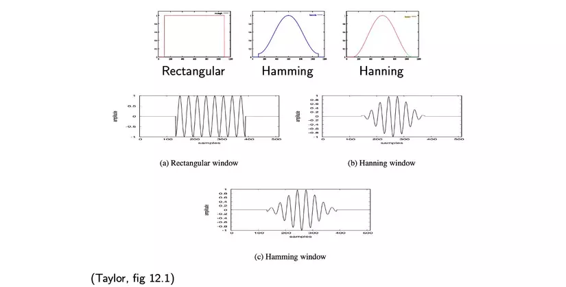
The following image shows the effect of these windows. In the thumbnails, Figure 1 is the frame cut from the original audio, the original sound is a combination of 2 wave 2. If the rectangle window is applied (ie direct cut), the corresponding frequency domain signal As shown in Figure 3, we can see this signal contains a lot of noise. If we apply windows like Hanning, Hamming, Blackman, the frequency domain signal is quite smooth and the original wave in Figure 2. 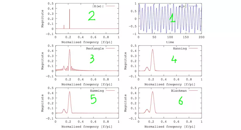
2.2 DFT
On each frame, we apply DFT – Discrete Fourier Transform by the formula:

Each frame we get a list of magnitude values corresponding to each word frequency 0 → N 0 to N 0 → N. Apply on all frames, we have obtained 1 Spectrogram as shown below. Axis x x x is the time axis (corresponding to the order of the frames), the axis y y y represents the magnetic frequency range 0 → 10000 0 to 10000 0 → 1 0 0 0 0 Hz, magnitude values at each frequency are shown in color. By observing this spectrogram, we find that the low frequencies often have high magnitude, high frequencies often have low magnitude.
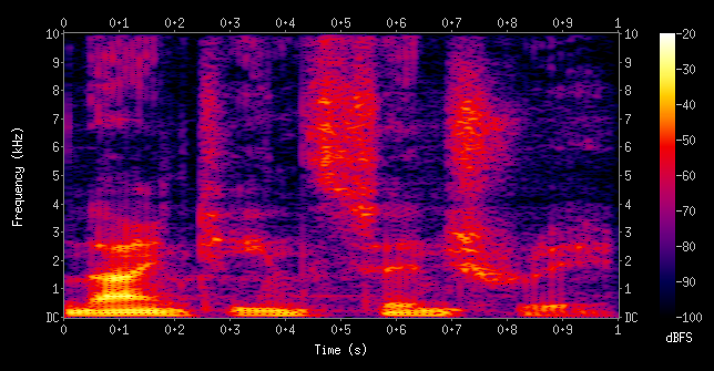
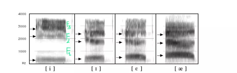
The picture below is the spectrogram of 4 vowels. Observing the spectrogram from the bottom up, it was found that there are several characteristic frequencies called formsant , called frequencies F1, F2, F3 … The phonetic experts can rely on the position, time, change of the formant on the spectrogram to determine which sound clip is which phoneme.
So we know how to create spectrogram. However, in many problems (especially speech recognition), spectrogram is not a perfect choice. So we need a few more calculation steps to get the MFCC form, better, more common, more efficient than spectrogram.
3. Mel filterbank
As I described in the previous section, the way the human ear feels is nonlinear, unlike measuring devices. The human ear feels good at low frequencies, less sensitive to high frequencies. We need a similar mapping mechanism.
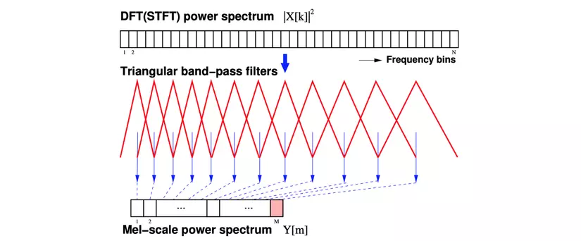
First, we square the values in the spectrogram to obtain the DFT power spectrum . Then, we apply a set of Mel-scale filter bandwidth filters on each frequency range (each filter applies on a specific frequency range). The output value of each filter is the frequency range energy that the filter covers (covers). We obtained Mel-scale power spectrum . In addition, filters for the low frequency range are often narrower than the filters for the high frequency range.
This process can also be described by the following illustration: 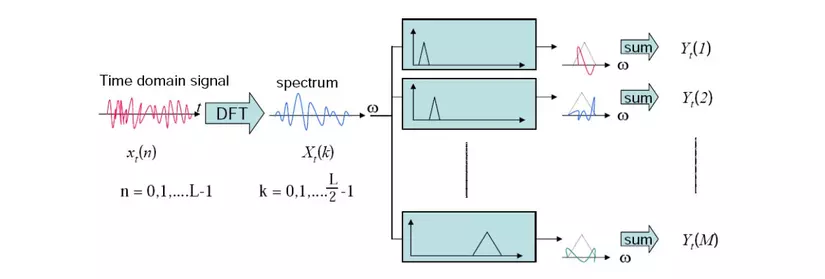
4. Cepstrum
4.1 Log
Mel filterbank returns the power spectrum of the sound, or energy spectrum. The fact that humans are less sensitive to energy changes at high frequencies is more sensitive at low frequencies. So we will calculate the log on the Mel-scale power spectrum. This also helps reduce insignificant sound variations for speech recognition.
4.2 IDFT – Inverse DFT
As described earlier, our voice frequency F0 – fundamental frequency and formant F1, F2, F3 … Frequency F0 male about 125 Hz, 210 Hz in women, particularly represents the pitch of the voice in each person. This pitch information is not useful in speech recognition, so we need to find a way to eliminate information about F0, helping the recognition model not depend on individual voice pitch.
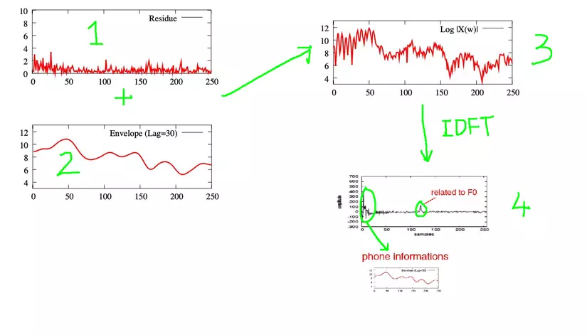
In this picture, the signal we get is graph 3, but the important information we need is part 2, the information we need to remove is part 1. To remove information about F0, we take 1 variable step converting Fourier backwards (IDFT) to the time domain, we obtain Cepstrum. If you look closely, you will realize that the name ” cepstrum ” actually reverses the first four letters of ” spetrum “.
Then, with Cepstrum obtained, the information related to F0 and the information related to F1, F2, F3 … are separated as two circles in Figure 4. We simply get the information. in the first paragraph of cepstrum (the large circle in Figure 4). To calculate MFCC, we only need the first 12 values.
IDFT transform is equivalent to a DCT discrete cosine transformation . DCT is an orthogonal transformation. Mathematically, this transformation creates uncorrelated features , which can be interpreted as independent or poorly correlated features. In Machine learning algorithms, uncorrelated features often give better results. So after this step, we get 12 Cepstral features.
5. MFCC
Thus, each frame we have extracted 12 Cepstral features as the first 12 features of MFCC. The 13th feature is the energy of that frame, calculated by the formula: 
In speech recognition, information about context and change is important. For example, at the beginning or ending points of many consonants, this change is very pronounced and can identify phonemes based on this change. The next 13 coefficients are the first derivatives (over time) of the first 13 features. It contains information about the change from th frame t t t to frame t + first t + 1 t + 1 . Recipe:
d ( t ) = c ( t + first ) – c ( t – first ) 2 d (t) = frac {c (t + 1) – c (t-1)} {2} d ( t ) = 2 c (t + 1) – c (t – 1)
Similarly, the last 13 values of MFCC are variable d ( t ) DT) d ( t ) over time – the derivative of d ( t ) DT) d ( t ) , is also the second derivative of c ( t ) c (t) c ( t ) . Recipe:
b ( t ) = d ( t + first ) – d ( t – first ) 2 b (t) = frac {d (t + 1) – d (t-1)} {2} b ( t ) = 2 d (t + 1) – d (t – 1)
Let’s look back at the whole process to create MFCC:
6. Conclusion
So in these 2 parts, I tried to provide the basic knowledge needed for speech processing. In the future, I will try to write about the speech recognition model Auto Speech Recognition (ASR), about HMM, GMM … and many other related things.
Margin:
I am the admin of the Vietnam AI Link Sharing Community group : a community specializing in sharing, exchanging in depth about papers, algorithms, author, competition or. Here the community will have access to more in-depth knowledge, not being diluted, drifting, lack of missing posts in common groups. We hope everyone will visit, if possible, join and build a strong community. Thank you everyone for reading.
Link: Vietnam AI Link Sharing Community