1. Entropy

1.1 Information theory and entropy

Information Theory – Information theory is a branch of mathematics involved in measuring, quantifying, and coding information. Information Theory’s father is Claude Shannon. He studies how to encode information when transmitting, so that the communication process is most effective without losing information.

H1: Claude Shannon

In 1948, in one of his essays, Claude Shannon referred to the concept of information entropy as a measure to quantify information or its uncertainty / uncertainty. There are many ways to translate entropy: uncertainty, chaos, uncertainty, surprise, unpredictability … of information. In this article, I will keep the word entropy instead of translating it into Vietnamese.

To make it easier to understand, I will take an example as follows: suppose after observing the weather for 1 year, you can record the following information:

• In winter, the probability of a sunny (light) day is 100% and the probability of a rainy day is 0%. So based on that probability, in winter we can confidently predict whether it will rain or shine tomorrow. In this case, the certainty is high, it’s not surprising that it won’t rain tomorrow.
• In the summer, the probability of a day without rain is 50%, with rain is 50%. Thus, the probability of rain / sunshine is the same. It is very difficult to predict whether tomorrow will be rainy or sunny, the certainty is not high. In other words, the rain or the sun tomorrow is more surprising in case 1.
• Thus, we need a mechanism to measure information uncertainty, in other words, to measure the amount of information.

Through the above example, we have a clearer view of the concept of entropy.

1.2 Entropy and information encryption

1.2.1 Encoding information

To better understand the concept, applicability, and computation of entropy, let’s first take a look at the topic of coding information.

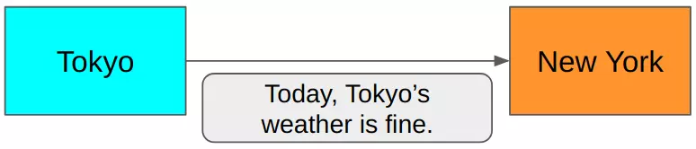
Suppose that when transmitting the weather from Tokyo to New York, assuming both sides already know that the message is just a rain / shine issue of Tokyo. We can send the message “Tokyo, Tokyo’s weather is fine”. However, it seems this way is a bit redundant. Since both Tokyo and New York bridge points know that the incoming / outgoing information is about the Tokyo weather. That means that Tokyo spot just transmits 1 in 2 rain-and-hot messages is enough for people in New York to understand. This way sounds quite reasonable, but still not optimal. The two sides only need to pre-convention with each other that: rain is 0, sunshine is 1. So the transmitted value only needs (0, 1) is enough. In this way, the transmitted information is optimized without fear of loss or misunderstanding between the sending / receiving parties.

With the above encryption method, we used 1 bit to encrypt the information. In binary, 1 bit will have the value 0 or 1. Below is a model for encoding and transmitting information. Information is encrypted (according to a conventional encoding) before being transmitted. At the receiving point, the receiver will receive the encrypted information, at which point the receiver needs to decode it to get the original information.

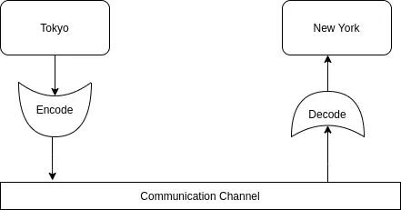
Simple encryption and information transmission model

1.2.2 Entropy

Medium encoding size

We have understood how to encode information. So how to compare the efficiency of encoding with two different encodings. In other words, how to determine which charset is better. Please observe the image below.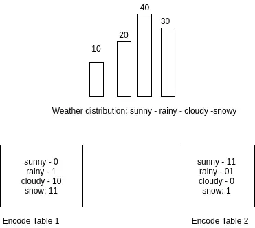

H4. Weather frequency statistics table and two different coding methods.

Note: when coding, the leading zeros will be omitted, for example: 001 -> 1, 0000100 -> 100 …

Suppose, after 100 weather records in Tokyo, the distribution as shown above is obtained with the frequency of sunshine-rain-cloud-snow 10, 20, 40, 30 times respectively. We have two encoding tables as shown in the picture. To compare the efficiency of the two encodings above, we compare the average number of bits transmitted per transmission.

• Code table 1: everage_bit = ( ten ∗ first + 20 ∗ first + 40 ∗ 2 + 30 ∗ 2 ) / 100 = 1.7 (10 * 1 + 20 * 1 + 40 * 2 + 30 * 2) / 100 = 1.7 $(10\ast 1+20\ast 1+40\ast 2+30\ast 2)/100=1.7$ bits.
• Code table 2: everage_bit = ( ten ∗ 2 + 20 ∗ 2 + 40 ∗ first + 30 ∗ first ) / 100 = 1.1 (10 * 2 + 20 * 2 + 40 * 1 + 30 * 1) / 100 = 1.1 $(10\ast 2+20\ast 2+40\ast 1+30\ast 1)/100=1.1$ bit

In the field of encoding, encoding 2 is considered to be more optimal than encoding 1 because if using encoding 2 will save more bits, spend less bandwidth (when transmitting) or take up less space ( storage). The above calculation is called the average encoding size calculation

e v e r a g e B i t = p first ∗ n first + p 2 ∗ n 2 + . . . + p k ∗ n n everageBit = p_1 * n_1 + p2 * n_2 + … + p_k * n_n e v e r a g e B i t = p 1 ∗ n 1 + p 2 ∗ n 2 + . . . + p k ∗ n n

( first ) (first) $$(1)$$

With n i n_i n i is the number of bits used to encode a frequency signal $p$ $i$ $p\_i$ p i

Minimum average encoding size

So how to choose the most optimal encoding. We need to choose an encoding that has the smallest average encoding size.

Just now is a simple example of a weather topic with 4 types of messages (sunshine, rain, clouds, snow) that need to be encoded, we only need to use 2 bits to encode these 4 types of messages. Similar to N messages, we need the number of bits encoded as:

n = log ⁡ 2 N n = log_2 ^ N n = lo g 2 N

Assume 1 of these messages have the same frequency p = first / N p = 1 / N $p=1/N.$

n p = log ⁡ 2 N = log ⁡ 2 first p = – log ⁡ 2 p n_p = log_2 ^ N = log_2 ^ frac {1} {p} = – log_2 ^ p n p = lo g 2 N = lo g 2 p 1 = – lo g 2 p

So – log ⁡ 2 P – log_2 ^ {P} – lo g 2 P is the minimum number of bits to encode a message with the probability of occurrence $p$ $p$ p . Combined with formula (1), we get the formula to calculate the minimum average encoding size , this is the Entropy formula:

E n t r o p y = – ∑ i n p i ∗ n i = – ∑ i n p i ∗ log ⁡ 2 p i Entropy = – sum_ {i} ^ {n} p_i * n_i = – sum_ {i} ^ {n} p_i * log_2 ^ {p_i} E n t r o p y = – i Σ n p i ∗ n i = – i Σ n p i ∗ lo g 2 p i

In fact, we can change log ⁡ 2 log_2 lo g 2 equal $log$ $$ $ten$ $log\_\; \{10\}$ lo g 1 0 , $log$ $$ $e$ $log\_e$ lo g e ..

Conclusion : entropy tells us the theoretical minimum coding size for events that follow a particular probability distribution.

Entropy properties.

With the above entropy formula, entropy is calculated entirely from probability. Suppose with a probability distribution of weather (rain, sunshine) P = {p1, p2}. It is recognized that Entropy (P) reaches max when p1 = p2. When p1 and p2 are different from each other, Entropy (P) decreases. If p1 = p2 = 0.5, entropy reaches max, it is very difficult to predict tomorrow weather is rainy or sunny. If p1 = 0.1 and p2 = 0.9, we would confidently predict that it would be sunny tomorrow, and the entropy would have a much lower value.

High entropy means it is difficult to predict an impending event. We can call it uncertainty, instability or entropy is a measure of the “unpredictability” of information.

2. Cross Entropy

As defined above, entropy is the theoretical minimum coding size for events subject to a particular probability distribution. As long as we know the distribution, we will get Entropy.

However, we are not always aware of that distribution. As the weather example in part 1, the distribution we use is essentially just the distribution we get from a statistic of the series of events that happened in the past. We cannot guarantee that the weather next year will be the same as last year. In other words, the distribution obtained from the statistics of the past is only approximate, approximate the actual distribution of the signal future.

To make it easier to understand, I will take the following example of the weather:

• At the beginning of 2019, the weather statistics for the whole year of 2018 were reported and the distribution obtained (sunshine, rain, clouds, snow) was Q = {0.1, 0.3, 0.4, 0.2}
• People rely on Q to encode these 4 messages for the year to 2019. Q is called the estimated distribution. The messages are encrypted and will continue to be transmitted throughout 2019 from Tokyo to New York.
• By the end of 2019, the weather for the whole year was recorded again, resulting in a new distribution of P = {0.11, 0.29, 0.41, 0.19}. P is considered the correct distribution for 2019.

Thus, based on the formula demonstrated in part 1, the average number of bits used throughout 2019 is:

C r o S S E n t r o p y ( P , Q ) = – ∑ i n p i ∗ log ⁡ 2 q i CrossEntropy (P, Q) = – sum_ {i} ^ {n} p_i * log_2 ^ {q_i} C r o s s E n t r o p y ( P , Q ) = – i Σ n p i ∗ lo g 2 q i

Thus, the Entropy of this signal has P distribution (the expectation is based on P), but it is encoded based on the Q distribution. That’s why the name CrossEntropy was born (cross means cross , I don’t know how to translate for standards).

The special properties of CrossEntropy are that:

• hits a minimum value if P == Q
• Very sensitive to the difference between p i p_i p i and $q$ $i$ $q\_i$ q i . when the $p$ $i$ $p\_i$ p i and $q$ $I$ $q\_I$ q I the more the difference, the faster the cross_entropy value increases.

Because machine learning problems are routinely about model building problems so that the output is as close to the target as possible (output, the target is usually in the form of a probability distribution). Based on this sensitivity , people use CrossEntropy to optimize models.

3. KL Divergence

After going through the Cross Entropy section, you will find that KL Divergence is very simple.

Still with the weather example in Part 2. Suppose at the end of 2019 CrossEntropy (P, Q) is calculated. This time, we wanted to determine if they’ve spent, how much more damage when coding bits based on Q instead of P. We have:

D K L ( P ∣ ∣ Q ) = C r o S S E n t r o p y ( P , Q ) – E n t r o p y ( P ) D_ {KL} (P || Q) = CrossEntropy (P, Q) – Entropy (P) D K L ( P ∣ ∣ Q ) = C r o s s E n t r o p y ( P , Q ) – E n t r o p y ( P )

= – ∑ i n p i ∗ log ⁡ 2 q i + ∑ i n p i ∗ log ⁡ 2 p i = – sum_ {i} ^ {n} p_i * log_2 ^ {q_i} + sum_ {i} ^ {n} p_i * log_2 ^ {p_i} = – i Σ n p i ∗ lo g 2 q i + I Σ n p i ∗ lo g 2 p i

= ∑ i n p i ∗ log ⁡ 2 p i q i = sum_ {i} ^ {n} p_i * log_2 ^ { frac {p_i} {q_i}} = Σ i n p i ∗ lo g 2 q i p i

Thus, KL Divergence is a way to estimate losses , approximately 1 distribution of P equals the distribution of Q.

DL DIvergence Properties:

• There is no symmetry, ie D K L ( P ∣ ∣ Q ) ≠ D K L ( Q ∣ ∣ P ) D_ {KL} (P || Q) neq D_ {KL} (Q || P) D K L ( P ∣ ∣ Q )  = D K L ( Q ∣ ∣ P )
• Like CrossEntropy, DL is also very sensitive to the difference between p i p_i p i and $q$ $i$ $q\_i$ q i

In Machine Learning / Deep Learning problems, since Entropy (P) is constant (P is target distribution -> constant), KL_Divergence function optimization is equivalent to optimization of CrossEntropy function. In other words, whether you use KL_Divergence or CrossEntropy in Machine Learning is the same (not in other fields).

4. References

1. Machine learning summary fundamental – https://jonathan-hui.medium.com
2. KL Divergence Demystified – Medium.com
3. What is Cross-Entropy in Machine learning? – https://medium.com