In this article, I would like to introduce Dropout (Dropout) in Neural network, then I will have some code to see how Dropout affects the performance of Neural network.
1. Theory
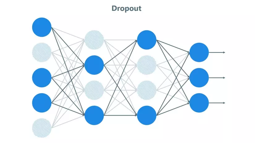
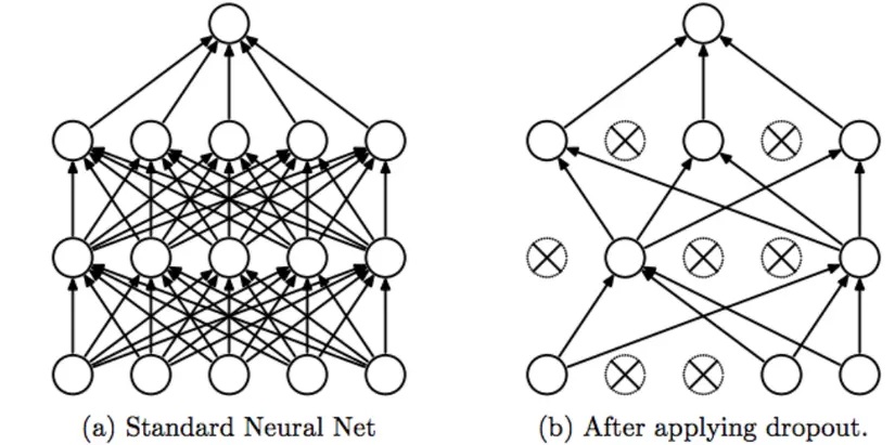
1.1. What is a dropout in a neural network?
According to Wikipedia – The term ‘Dropout’ refers to the ignoring of hidden and visible units in a Neural network.
Understand a simple way, the Dropout is ignoring the unit (ie a network node) in the training process randomly. By omitting this unit, the unit will not be considered during forward and backward. Accordingly, p is called the probability of retaining a network node during each training period, so the probability that it will be rejected is (1 – p).
1.2. Why need Dropout
The question is: Why do I have to literally turn off some network nodes during training? The answer is: Avoid Over-fitting.
If a fully connected class has too many parameters and takes up most of the parameters, the network nodes in that class are too interdependent during training, limiting each node’s power, leading to over-coupling .
1.3. Other techniques
If you want to know what Dropout is, just the above 2 theory parts are enough. In this part I also introduce a number of techniques that have the same effect with Dropout.
In Machine Learning, regularization reduces over-fitting by adding a range of ‘penalties’ to the loss function. By adding such a value, your model won’t learn too much of dependencies between the weights. Surely many people who know Logistic Regression know that L1 (Laplacian) and L2 (Gaussian) are two ‘penalty’ techniques.
- Training process: For each hidden layer, example, per loop, we will drop out randomly with probability (1 – p) for each network node.
- Test Process: Use all triggers, but will decrease by 1 p-factor (to account for dropped actives).

1.4. Some comments
- Dropout will learn more powerful useful features
- It almost doubles the number of epochs needed to converge. However, the time per epoch is less.
- We have H hidden units, with the dropout probability for each unit of (1 – p) we can have 2 ^ H possible models. But during the test phase, all network nodes must be considered, and each activation will be reduced by a factor p.
2. Practice
Talking is a bit confusing, so I will code 2 parts to see what Dropout is like.
Problem: You go to a football match and you try to predict where the goalkeeper takes a shot and the home player hits the ball.
I imported the necessary libraries
1 2 3 4 5 6 7 8 9 10 11 12 13 14 15 16 | # import packages import numpy as np import matplotlib.pyplot as plt from reg_utils import sigmoid, relu, plot_decision_boundary, initialize_parameters, load_2D_dataset, predict_dec from reg_utils import compute_cost, predict, forward_propagation, backward_propagation, update_parameters import sklearn import sklearn.datasets import scipy.io from testCases import * %matplotlib inline plt.rcParams['figure.figsize'] = (7.0, 4.0) # set default size of plots plt.rcParams['image.interpolation'] = 'nearest' plt.rcParams['image.cmap'] = 'gray' |
Visualize the data a bit
1 2 | train_X, train_Y, test_X, test_Y = load_2D_dataset() |
We get results
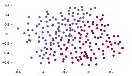
The red dot is the home player who has hit his head, the green dot is the player you hit. What we do is predict which area the goalkeeper should shoot the ball into so that the home player can hit his head. Looks like you only need to draw a line to divide the 2 areas.
2.1. The model does not have formalization
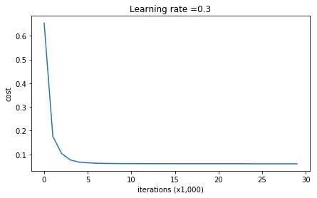
1 2 3 4 5 6 7 8 9 10 11 12 13 14 15 16 17 18 19 20 21 22 23 24 25 26 27 28 29 30 31 32 33 34 35 36 37 38 39 40 41 42 43 44 45 46 47 48 49 50 51 52 53 | def model(X, Y, learning_rate = 0.3, num_iterations = 30000, print_cost = True): """ Triển khai mạng với 3 layer: LINEAR->RELU->LINEAR->RELU->LINEAR->SIGMOID. Tham số: X -- Dữ liệu đầu vào, kích thước (input size, number of examples) Y -- 1 vector (1 là chấm xanh / 0 là chấm đỏ), kích thước (output size, number of examples) learning_rate -- Tỷ lệ học num_iterations -- Số epochs print_cost -- Nếu là True, in ra coss cho mỗi 10000 vòng lặp Returns: parameters -- Tham số học được, được dùng để dự đoán """ grads = {} costs = [] # to keep track of the cost m = X.shape[1] # number of examples layers_dims = [X.shape[0], 20, 3, 1] # Initialize parameters dictionary. parameters = initialize_parameters(layers_dims) # Loop (gradient descent) for i in range(0, num_iterations): # Forward propagation: LINEAR -> RELU -> LINEAR -> RELU -> LINEAR -> SIGMOID. a3, cache = forward_propagation(X, parameters) # Cost function cost = compute_cost(a3, Y) grads = backward_propagation(X, Y, cache) # Update parameters. parameters = update_parameters(parameters, grads, learning_rate) # Print the loss every 10000 iterations if print_cost and i % 10000 == 0: print("Cost after iteration {}: {}".format(i, cost)) if print_cost and i % 1000 == 0: costs.append(cost) # plot the cost plt.plot(costs) plt.ylabel('cost') plt.xlabel('iterations (x1,000)') plt.title("Learning rate =" + str(learning_rate)) plt.show() return parameters |
Prediction function
1 2 3 4 5 | print("On the training set:") predictions_train = predict(train_X, train_Y, parameters) print("On the test set:") predictions_test = predict(test_X, test_Y, parameters) |
See the results
1 2 3 4 5 6 7 8 9 | Cost after iteration 0: 0.6557412523481002 Cost after iteration 10000: 0.16329987525724216 Cost after iteration 20000: 0.13851642423255986 ... On the training set: Accuracy: 0.947867298578 On the test set: Accuracy: 0.915 |
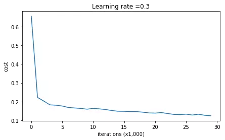
It can be seen that the training accuracy is 94% and the test set is 91% (quite high). We’ll visualize a bit
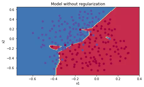
When there is no formalization, we see a very detailed draw line, that is, it is over-fitting.
2.2. Regularized model with Dropout
2.2.1. Forward Propagation process
1 2 3 4 5 6 7 8 9 10 11 12 13 14 15 16 17 18 19 20 21 22 23 24 25 26 27 28 29 30 31 32 33 34 35 36 37 38 39 40 41 42 43 44 45 46 47 48 49 50 51 52 53 54 | def forward_propagation_with_dropout(X, parameters, keep_prob=0.5): """ Triển khai 3 layer: LINEAR -> RELU + DROPOUT -> LINEAR -> RELU + DROPOUT -> LINEAR -> SIGMOID. Arguments: X -- Dữ liệu đầu vào, kích thước (2, number of examples) parameters -- Các đối số chúng ta có "W1", "b1", "W2", "b2", "W3", "b3": W1 -- weight matrix of shape (20, 2) b1 -- bias vector of shape (20, 1) W2 -- weight matrix of shape (3, 20) b2 -- bias vector of shape (3, 1) W3 -- weight matrix of shape (1, 3) b3 -- bias vector of shape (1, 1) keep_prob - xác suất giữ lại 1 unit Returns: A3 -- giá trị đầu ra mô hình, kích thước (1,1) cache -- lưu các đối số để tính cho phần Backward Propagation """ np.random.seed(1) # retrieve parameters W1 = parameters["W1"] b1 = parameters["b1"] W2 = parameters["W2"] b2 = parameters["b2"] W3 = parameters["W3"] b3 = parameters["b3"] # LINEAR -> RELU -> LINEAR -> RELU -> LINEAR -> SIGMOID Z1 = np.dot(W1, X) + b1 A1 = relu(Z1) ### START CODE HERE ### (approx. 4 lines) # Steps 1-4 below correspond to the Steps 1-4 described above. D1 = np.random.rand(A1.shape[0], A1.shape[1]) # Step 1: khởi tạo ngẫu nhiên 1 ma trận kích thước bằng kích thước A1, giá trị (0, 1) D1 = D1 < keep_prob # Step 2: chuyển các giá trị về 0 hoặc 1, trả về 1 nếu giá trị đó nhỏ hơn keep_prob A1 = A1 * D1 # Step 3: giữ nguyên các phần tự trong A1 ứng với phần tử 1 của D1, và đổi thành 0 nếu vị trị trong D1 tương tứng là 0 A1 = A1 / keep_prob # Step 4: giảm đi 1 hệ số keep_prob, để tính cho các phần tử đã bỏ học. ### END CODE HERE ### Z2 = np.dot(W2, A1) + b2 A2 = relu(Z2) ### START CODE HERE ### (approx. 4 lines) D2 = np.random.rand(A2.shape[0], A2.shape[1]) D2 = D2 < keep_prob A2 = A2 * D2 A2 = A2 / keep_prob ### END CODE HERE ### Z3 = np.dot(W3, A2) + b3 A3 = sigmoid(Z3) cache = (Z1, D1, A1, W1, b1, Z2, D2, A2, W2, b2, Z3, A3, W3, b3) return A3, cache |
2.2.2. Backward Propagation process
1 2 3 4 5 6 7 8 9 10 11 12 13 14 15 16 17 18 19 20 21 22 23 24 25 26 27 28 29 30 31 32 33 34 35 36 37 38 39 40 41 | def backward_propagation_with_dropout(X, Y, cache, keep_prob): Các đối số: X -- Dữ liệu đầu vào, kích thước (2, number of examples) Y -- kích thước (output size, number of examples) cache -- lưu đầu ra của forward_propagation_with_dropout() keep_prob - như forward Returns: gradients -- Đạo hàm của tất cả các weight, activation """ m = X.shape[1] (Z1, D1, A1, W1, b1, Z2, D2, A2, W2, b2, Z3, A3, W3, b3) = cache dZ3 = A3 - Y dW3 = 1. / m * np.dot(dZ3, A2.T) db3 = 1. / m * np.sum(dZ3, axis=1, keepdims=True) dA2 = np.dot(W3.T, dZ3) ### START CODE HERE ### (≈ 2 lines of code) dA2 = dA2 * D2 # Step 1: Áp dụng D2 để tắt các unit tương ứng với forward dA2 = dA2 / keep_prob # Step 2: Giảm giá trị 1 hệ số keep_prob ### END CODE HERE ### dZ2 = np.multiply(dA2, np.int64(A2 > 0)) dW2 = 1. / m * np.dot(dZ2, A1.T) db2 = 1. / m * np.sum(dZ2, axis=1, keepdims=True) dA1 = np.dot(W2.T, dZ2) ### START CODE HERE ### (≈ 2 lines of code) dA1 = dA1 * D1 dA1 = dA1 / keep_prob ### END CODE HERE ### dZ1 = np.multiply(dA1, np.int64(A1 > 0)) dW1 = 1. / m * np.dot(dZ1, X.T) db1 = 1. / m * np.sum(dZ1, axis=1, keepdims=True) gradients = {"dZ3": dZ3, "dW3": dW3, "db3": db3,"dA2": dA2, "dZ2": dZ2, "dW2": dW2, "db2": db2, "dA1": dA1, "dZ1": dZ1, "dW1": dW1, "db1": db1} return gradients |
After having Forward and Backward, we replace these 2 functions in the model function of the previous section:
1 2 3 4 5 6 7 | parameters = model(train_X, train_Y, keep_prob=0.86, learning_rate=0.3) print("On the train set:") predictions_train = predict(train_X, train_Y, parameters) print("On the test set:") predictions_test = predict(test_X, test_Y, parameters) |
Result:
1 2 3 4 5 6 7 8 | Cost after iteration 10000: 0.06101698657490559 Cost after iteration 20000: 0.060582435798513114 ... On the train set: Accuracy: 0.928909952607 On the test set: Accuracy: 0.95 |
We see, the test set accuracy was up to 95%, although the training training was reduced. Perform visualize:
1 2 3 4 5 6 | plt.title("Model with dropout") axes = plt.gca() axes.set_xlim([-0.75, 0.40]) axes.set_ylim([-0.75, 0.65]) plot_decision_boundary(lambda x: predict_dec(parameters, x.T), train_X, train_Y) |
We can 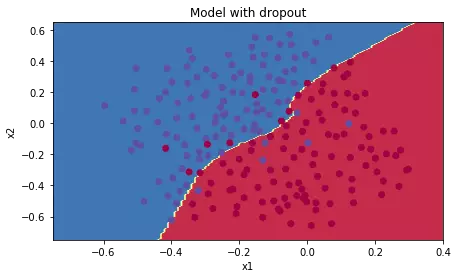
We see that the dividing line is not too detailed, so over-fitting is avoided.
2.3. Attention
- Do not use Dropout for the test
- Apply Dropout for both Forward and Backward
- The trigger value must be reduced by 1 keep_prob factor, including dropout nodes.
Source: Medium