Hello everyone to see you again =))). In this Viblo article, I will share about a problem that most E-commerce websites need – Customer Segmentation. However, I will use the ML model to solve this problem .
Customer segmentation is the finding and selection of groups of customers that businesses and organizations are able to satisfy needs better than competitors. His reference here
Purpose:
- To choose the right customers and serve the best way
- Create a competitive advantage with competitors in the market
- Understanding customers and affirming the brand Ways to segment customers that businesses are currently doing:
- Geography
- Sex
- Age
- Income.
Customer segmentation applies ML
Data
Here I have used data based on data of an e-commerce site on customer transactions, people can download it here.
Read the data to see what our data has.
1 2 3 4 5 6 | import pandas as pd dataset = pd.read_csv('customerSpending.csv', header = 0, index_col = 0) print(dataset.shape) dataset.head() |
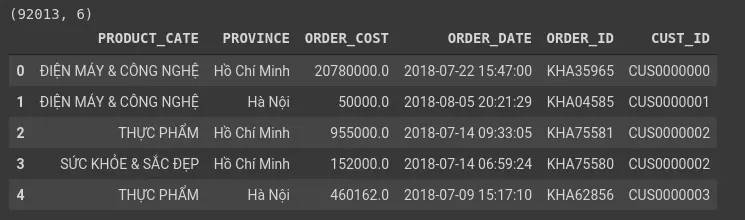
Our data includes the fields:
- PRODUCT_CATE: The type of transaction product
- PROVINCE: transaction provinces
- ORDER_COST: Product price
- ORDER_DATE: Order time
- ORDER_ID: order code
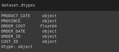
- CUST_ID: Customer ID The data format of the fields:
 Here the ORDER_ID field is the most important.
Preprocessing Data
Processing and converting data
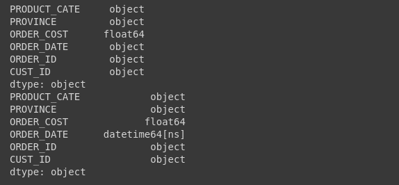
First we will convert datetime from Object to Datetime64 format.
1 2 3 4 5 6 7 8 9 | from datetime import datetime def strToDatetime(x): return datetime.strptime(x, '%Y-%m-%d %H:%M:%S') # Kiểm tra định dạng các trường của pandas dataframe print(dataset.dtypes) # Convert dữ liệu về đúng định dạng dataset['ORDER_DATE'] = dataset['ORDER_DATE'].apply(strToDatetime) dataset.dtypes |
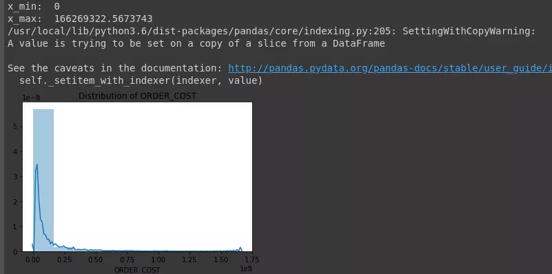
Next, we will try to draw a distribution chart of variables (bins = 10)
1 2 3 4 5 6 7 8 9 10 11 12 13 14 | # Thống kê mô tả print(dataset.describe()) # Vẽ biểu đồ phân phối các biến import seaborn as sns import matplotlib.pyplot as plt def plotNumeric(colname, n_bins = 10, hist = True, kde = True): sns.distplot(dataset[colname], hist = hist, kde = kde, bins = n_bins) plt.title('Distribution of {}'.format(colname)) plt.show() plotNumeric('ORDER_COST', hist = True, kde = True, n_bins = 10) |
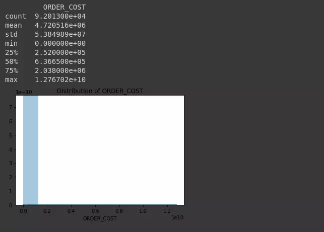
Determine the outlier points of the order value variable “ORDER_COST” based on the 3 sigma principle. According to the 3 sigma principle, 99.75% of the order value will range from:
[ μ – 3 σ , μ + 3 σ ] [ mu – 3 sigma, mu + 3 sigma]
Outliers are points that are located outside the upper range.
1 2 | dataset.loc[[1, 2]]['ORDER_COST'] |
1 2 3 4 5 6 7 8 9 10 11 12 13 14 15 | def fillOutlier(colname): mu = np.mean(dataset[colname]) sigma = np.std(dataset[colname]) x_min = max(mu - 3*sigma, 0) x_max = mu + 3*sigma print('x_min: ', x_min) print('x_max: ', x_max) out_lower_id = dataset[dataset[colname] < x_min].index out_upper_id = dataset[dataset[colname] > x_max].index dataset[colname].loc[out_lower_id] = x_min dataset[colname].loc[out_upper_id] = x_max fillOutlier('ORDER_COST') plotNumeric('ORDER_COST', hist = True, kde = True, n_bins = 10) |
Statistics of total values according to “PRODUCT_CATE” corresponding to “CUST_ID”.
1 2 3 4 5 6 7 8 9 10 | dfSummary = pd.pivot_table(data = dataset, values = ['ORDER_COST', 'ORDER_ID'], index = ['CUST_ID'], columns = ['PRODUCT_CATE'], aggfunc= {'ORDER_COST': np.sum} ) print(dfSummary.shape) dfSummary.head() |
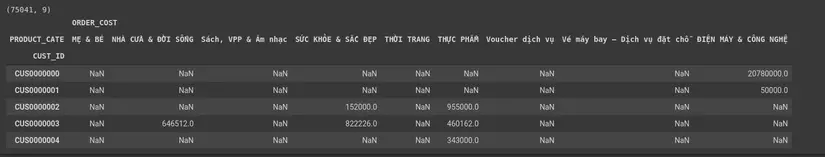
After the statistics are complete, we will fill in the na values, here we fillna with 0 home.
1 2 3 4 5 6 7 8 | from sklearn.preprocessing import StandardScaler dfSummary.fillna(0, inplace = True) scaler = StandardScaler() scaler.fit(dfSummary) X = scaler.transform(dfSummary) |
Training Model
Divide the train training and test practice with my family.
1 2 3 4 5 | from sklearn.model_selection import train_test_split X_train, X_test, id_train, id_test = train_test_split(X, np.arange(X.shape[0]), test_size = 0.2) |
Building Kmeans model, everyone can refer to KMean here
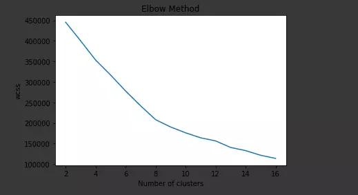
1 2 3 4 5 6 7 8 9 10 11 12 | from sklearn.cluster import KMeans # Khởi tạo mô hình kmean cluster với số cluster từ 2->16 kmeans = [] wcss = [] for i in np.arange(2, 17, 1): km_i = KMeans(n_clusters=i,init='k-means++', max_iter=300, n_init=10, random_state=0) km_i.fit(X_train) wcss.append(km_i.inertia_) kmeans.append(km_i) |
wcss: measure the deviation to centerpoints. When making the number of clussters makes the index of wcss insignificant, we can choose
1 2 3 4 5 6 7 8 | # Vẽ biểu đồ wcss vs n_clusters plt.plot(np.arange(2, 17),wcss) plt.title('Elbow Method') plt.xlabel('Number of clusters') plt.ylabel('wcss') # plt.ylim(0, 800000) plt.show() |
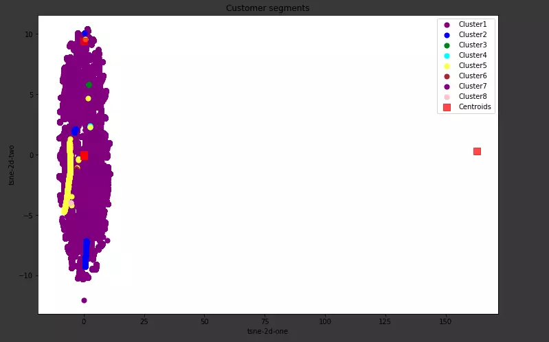
Visualize clusters: First we use tnse to reduce the data dimension from 9 to 2:
1 2 3 4 5 6 | from sklearn.manifold import TSNE import time time_start = time.time() tsne = TSNE(n_components=2, verbose=1, perplexity=40, n_iter=300) tsne_results = tsne.fit_transform(X_train) |
Next is Visualize:
1 2 3 4 5 6 7 8 9 10 11 12 13 14 15 16 17 18 19 20 21 | X_ = tsne_results y_label = kmeans[7].predict(X_train) plt.figure(figsize = (12, 8)) plt.scatter(X_[y_label==0,0],X_[y_label==0,1],s=50, c='purple',label='Cluster1') plt.scatter(X_[y_label==1,0],X_[y_label==1,1],s=50, c='blue',label='Cluster2') plt.scatter(X_[y_label==2,0],X_[y_label==2,1],s=50, c='green',label='Cluster3') plt.scatter(X_[y_label==3,0],X_[y_label==3,1],s=50, c='cyan',label='Cluster4') plt.scatter(X_[y_label==4,0],X_[y_label==4,1],s=50, c='yellow',label='Cluster5') plt.scatter(X_[y_label==5,0],X_[y_label==5,1],s=50, c='brown',label='Cluster6') plt.scatter(X_[y_label==6,0],X_[y_label==6,1],s=50, c='purple',label='Cluster7') plt.scatter(X_[y_label==7,0],X_[y_label==7,1],s=50, c='pink',label='Cluster8') # plt.scatter(X_[y_label==8,0],X_[y_label==8,1],s=50, c='orange',label='Cluster9') # plt.scatter(X[y_means==4,0],X[y_means==4,1],s=50, c='yellow',label='Cluster5') # plt.scatter(kmeans_7.cluster_centers_[:,0], kmeans_7.cluster_centers_[:,1],s=100,marker='s', c='red', alpha=0.7, label='Centroids') plt.scatter(kmeans[7].cluster_centers_[:,0], kmeans[7].cluster_centers_[:,1],s=100,marker='s', c='red', alpha=0.7, label='Centroids') plt.title('Customer segments') plt.xlabel('tsne-2d-one') plt.ylabel('tsne-2d-two') plt.legend() plt.show() |
Let’s see how the result looks like everyone:
Above, I use Kmeans to segment customers or people can refer to Anh Khanh’s article on RFM here using RFM (Recency – Frequency – Monetary model) model to segment customers by rank.
- VIP customers: rank from 8-10.
- Mass customers: rank from 5-7.
- Secondary customers: rank <5.
Please refer to the RFM code here
Conclude
The customer segmentation problem is quite common for TMTT to contribute correctly to customer needs. However, my problem is quite simple, hope that everyone can give me suggestions for my writing.
Reference
https://machinelearningcoban.com/2017/01/01/kmeans/ https://phamdinhkhanh.github.io/2019/11/08/RFMModel.html