1. Regression
I started to wonder why there is a name regression. Along with searching the wiki and what I learned in the recent course I participated; I have come up with the origin of the most primitive names in Machine Learning.
Regression analysis is one of the most common methods used in statistical data analysis. The term “regression” is defined by the house of Francis Galton. Sir Francis Galton has studied and written a number of papers related to the inheritance process in which he observes and discovers a characteristic in the relationship between the height of one generation and the height of the next.
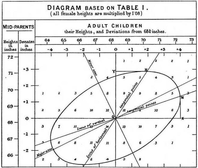
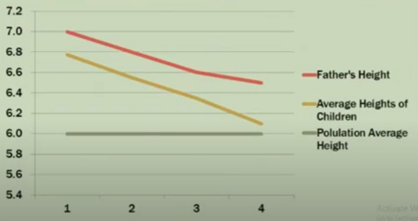
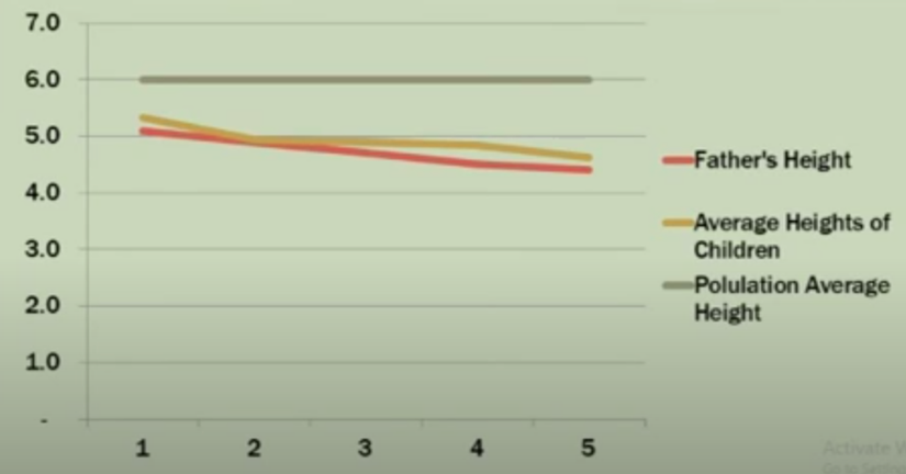
According to genetic theory, the previous generation with height greater than average will produce the next generation is also higher than average. However Francis found that the higher-than-average ratio of the next generation has decreased compared to the previous generation; At the same time, the following generations with lower average height tend to be the opposite, increasing compared to the previous generation.
Example of Galton’s pea experiment:
If the parent (F1) is 1.5 times larger than the F1 generation average. According to Galton’s theory, the (F2) will still be larger than the F2 generation average, but this size will tend to be 1.5 times smaller; and the exact opposite of smaller-than-average F1 generations. This interesting phenomenon is called by Galton Regression toward mean , which, according to him, dimensions always tend to return to the mean. The concept of Regression came from here
The image above is one of the first Linear regression models used by Galton in 1877 based on the pea size study.
Cool fact:
Fact 1 – Francis Galton is Charles Darwin’s cousin
Fact 2 – In fact, Francis Galton was not the first to apply the Linear regression model. One of the first founders of the regression model was mathematician Carl-Friedrich Gauss. Gauss invented the least square method to calculate the orbits of planets in astronomy.
Fact 3 – You can refer and use Peas Dataset in R
http://www.stat.uchicago.edu/~s343/Handouts/galton-peas.html https://www.picostat.com/dataset/r-dataset-package-psych-peas
2. Perceptron
One of the first foundations of neural networks and deep learning is the perceptron learning algorithm (or perceptron). Perceptron is a supervised learning algorithm that solves the binary classification problem, originated by Frank Rosenblatt in his research in 1957. The perceptron algorithm is proven to converge if two data layers are linearly separable .
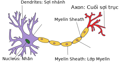
Perceptron’s idea is based on neurons in the brain. At the end of the neuron will contain the nucleus, the input signals through the dendrites (dendrites) and the output signals through the axon (axon) connected to other neurons. Simply understand, each neuron receives input data via branch fibers and transmits output data via axons, to the branch fibers of other neurons.
Each neuron receives electrical impulses from other neurons via branch fibers. If these electrical impulses are large enough to activate the neuron, this signal passes through the axon to the branch fibers of other neurons.
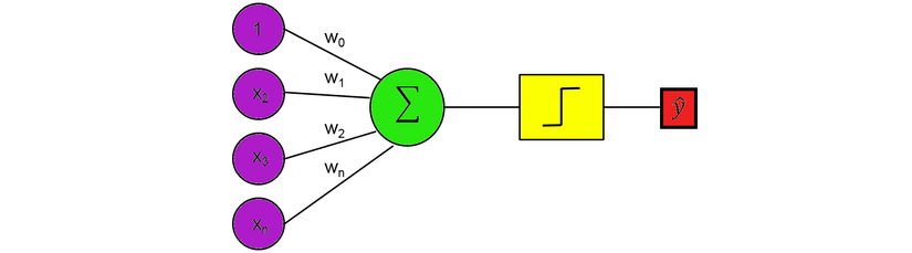
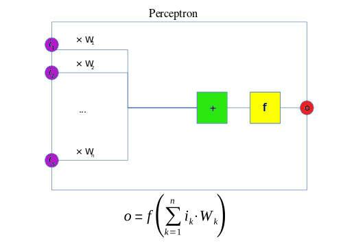
Single Layer Perceptron
This is a one-layer perceptron. It is like neurons, having inputs that then multiply by weight and sum all together. The value here is now compared to threshold and then converted using the activation function. For example, if the sum is greater than or equal to 0, then instantiate output to 1; otherwise, do not activate or output 0.
The inputs and the weights w act like neurotransmitters in a neuron, in which some can be positive and add to the sum, and some can be negative and subtracted from the sum. The function of the Unit Step Function acts as a threshold for the output.
If the threshold is met, then transmit the signal, otherwise the signal will not be transmitted.
Although this algorithm is promising, it has quickly been shown to be unable to solve simple problems. In 1969, Marvin Minsky and Seymour Papert in the famous book Perceptrons proved that it was impossible to “learn” the simple XOR function using the perceptron network.
3. Neural Network
Multi Layer Perceptron
The neuron output signal in the brain becomes the input signal for the next neuron, thereby forming reflexes that control the brain. The more complex the activity, the more neuron is needed. Therefore, forming a multi-layer network of single layter perceptrons will have a better learning model. However, if you combine multiple perceptron layers with the linear activation function, the output layer is still linear, the model will not learn much as a single layer perceptron. Therefore, with MLP the activation functions are selected as non-linear functions (sigmoid, fishy …)
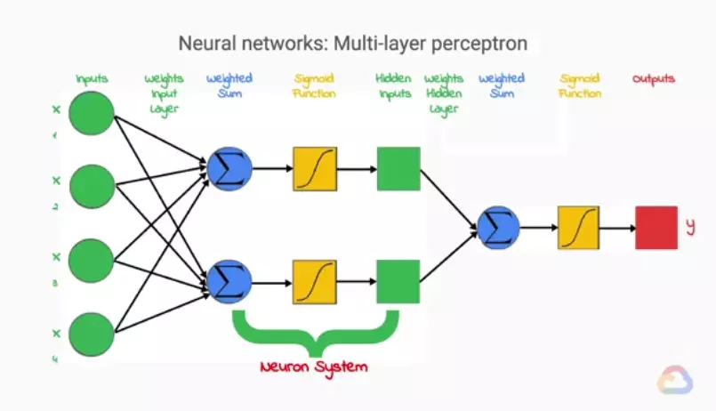
(Above image is taken from Machine Learning with TensorFlow on Google Cloud Platform)
Each output of a single perceptron layer becomes the input of another single perceptron layer, and is called Hidden inputs. And I’m going to go a little deeper into these layers. Each neuron we can understand is a set of 3 steps: Weight, activation function and output (hidden inputs). And together we have a hidden layer
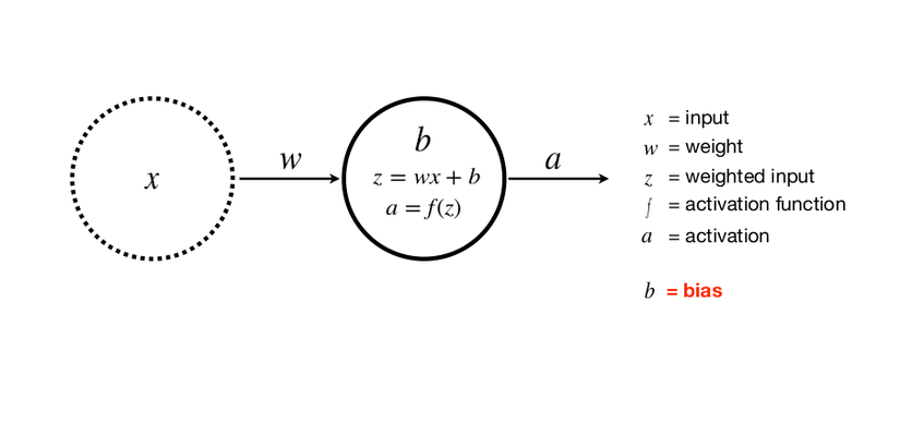
Where x is the input, w is the weight, z or y is the output, a is the activation class with f is the activation function
We have:
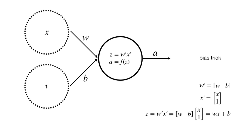
An input, a class, a neuron (where b is a bias). Adding bias helps to generalize the equation of the line, avoiding the case where the desired equation cannot be found
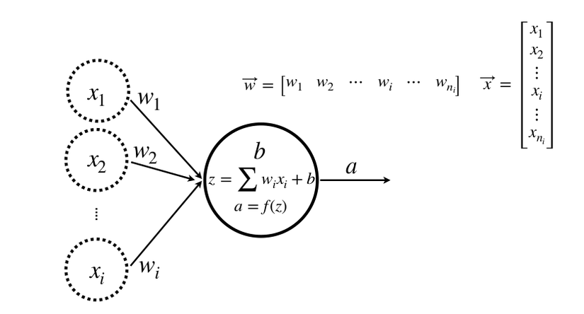
Multiple inputs, one class, one neuron
Multiple inputs, one class, many neurons
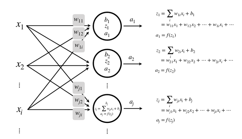
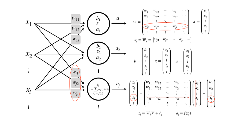
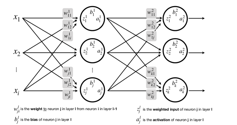
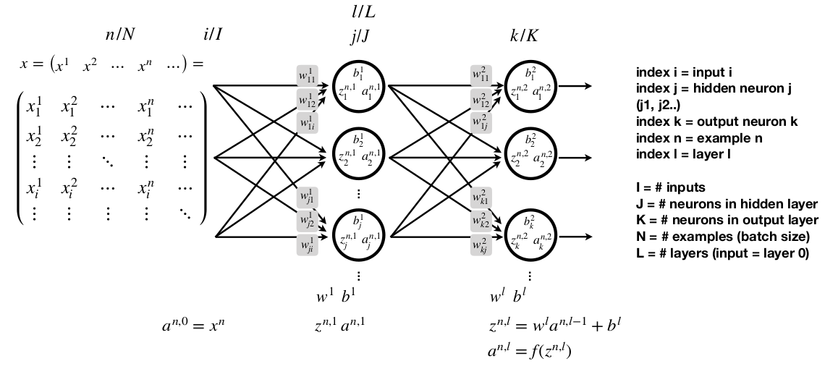
Multiple inputs, multiple layers, multiple neurons
And imagine if your input X is not a vector but a matrix image. It’s a lot more complicated, isn’t it?
With hidden layers, neural nets have been shown to be capable of approximating almost any function.
However, with MLP, there was a vanishing gradient problem due to the computing limitations of the time and the sigmoid function.
Conclusion
Learning about the world of Machine Learning is very interesting, I always have questions about the origin and the formation of current techniques. Today’s modern networks with more enhancements in computational power, data sources, ReLU functions with simple calculations and derivatives help significantly increase the training speed, Dropout techniques are used to increase calculation. generalization of the model … however, is still based on the previous Neural Network structure.
Reference source
https://en.wikipedia.org/wiki/Linear_regression
https://www.tandfonline.com/doi/full/10.1080/10691898.2001.11910537
https://www.youtube.com/watch?v=oEI0-kUmMJo&t=156s
https://machinelearningcoban.com/2018/06/22/deeplearning/
https://nttuan8.com/bai-3-neural-network/
Machine Learning with TensorFlow course on Google Cloud Platform Specialization on Coursera
Digital image Processing 3rd Edition by Rafael C. Gonzalez & Richard E. Woods Addison-Wesley
Special thanks to Prof. Frank Lindseth lectures